

244
WILLIAM STREIFER
4. Results
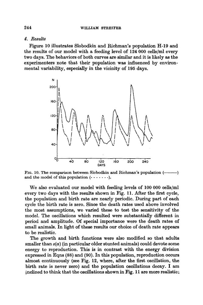
Figure 10 illustrates Slobodkin and Richman’s population H-19 and
the results of our model with a feeding level of 124 000 cellslml every
two days. The behaviors of both curves are similar and it is likely as the
experimenters note that their population was influenced by environmental variability, especially in the vicinity of 196 days.
I
O0
40
00
120
160
200
240
DAYS
FIU. 10. The comparison between Slobodkin and Richman’s population ( -
1
We also evaluated our model with feeding levels of 100 000 cellslml
every two days with the results shown in Fig. 11. After the first cycle,
the population and birth rate are nearly periodic. During part of each
cycle the birth rate is zero. Since the death rates used above involved
the most assumptions, we varied these to test the sensitivity of the
model. The oscillations which resulted were substantially different in
period and amplitude. Of special importance were the death rates of
small animals. I n light of these results our choice of death rate appears
to be realistic.
The growth and birth functions were also modified so that adults
smaller than s(a) (in particular older stunted animals) could devote some
energy to reproduction. This is in contrast with the energy division
expressed in Eqns (88) and (90). I n this population, reproduction occurs
almost continuously (see Fig. 12, where, after the first oscillation, the
birth rate is never zero) and the population oscillations decay. I am
inclined to think that the oscillations shown in Fig. 11 are more realistic;
and the model of this population (- - - - - - -).
WILLIAM STREIFER
4. Results
Figure 10 illustrates Slobodkin and Richman’s population H-19 and
the results of our model with a feeding level of 124 000 cellslml every
two days. The behaviors of both curves are similar and it is likely as the
experimenters note that their population was influenced by environmental variability, especially in the vicinity of 196 days.
I
O0
40
00
120
160
200
240
DAYS
FIU. 10. The comparison between Slobodkin and Richman’s population ( -
1
We also evaluated our model with feeding levels of 100 000 cellslml
every two days with the results shown in Fig. 11. After the first cycle,
the population and birth rate are nearly periodic. During part of each
cycle the birth rate is zero. Since the death rates used above involved
the most assumptions, we varied these to test the sensitivity of the
model. The oscillations which resulted were substantially different in
period and amplitude. Of special importance were the death rates of
small animals. I n light of these results our choice of death rate appears
to be realistic.
The growth and birth functions were also modified so that adults
smaller than s(a) (in particular older stunted animals) could devote some
energy to reproduction. This is in contrast with the energy division
expressed in Eqns (88) and (90). I n this population, reproduction occurs
almost continuously (see Fig. 12, where, after the first oscillation, the
birth rate is never zero) and the population oscillations decay. I am
inclined to think that the oscillations shown in Fig. 11 are more realistic;
and the model of this population (- - - - - - -).