

24
M. E. SOLOMON
level should not be too frequent. (Failing this condition, the method
could still provide the negative information that the population density
was not being uninterruptedly regulated towards any equilibrium level
that remained substantially the same over three or more census
intervals.) Nevertheless, under some conditions it might provide a
somewhat penetrating analysis of the dynamics of a population.
So far, only the prompt type of density-dependence has been considered. How does the method function if a population is involved in a
parasite-host cycle, so that the density-dependence operates with a lag
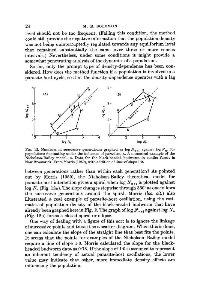
FIG. 12. Numbers in successive generations graphed as log N,,, against log N,, for
populations fluctuating under the influence of parasites. A. A numerical example of the
Nicholson-Bailey model. B. Data for the black-headed budworm in conifer forest in
New Brunswick. From Morris (1959), with addition of lines of slope 1.0.
between generations rather than within each generation? As pointed
out by Morris (1959), the Nicholson-Bailey theoretical model for
parasite-host interaction gives a spiral when log N,+l is plotted against
log N , (Fig. 1 2 ~ ) .
The slope changes stepwise through 360" as one follows
the successive generations around the spiral. Morris (Zoc. cit.) also
illustrated a real example of parasite-host oscillation, using the estimates of population density of the black-headed budworm that have
already beengraphed here in Fig. 2. The graph of log N,+l against log N ,
(Fig. 1 2 ~ )
forms a closed spiral or ellipse.
One way of dealing with a figure of this sort is to ignore the linkage
of successive points and treat it as a scatter diagram. When this is done,
one can calculate the slope of the straight line that best fits the points.
It seems that the points for examples of the Nicholson-Bailey model
require a line of slope 1.0. Morris calculated the slope for the blackheaded budworm data as 0.78. If the slope of 1.0 is assumed to represent
an inherent tendency of actual parasite-host oscillations, the lower
value may indicate that other, more immediate density effects are
influencing the population.
M. E. SOLOMON
level should not be too frequent. (Failing this condition, the method
could still provide the negative information that the population density
was not being uninterruptedly regulated towards any equilibrium level
that remained substantially the same over three or more census
intervals.) Nevertheless, under some conditions it might provide a
somewhat penetrating analysis of the dynamics of a population.
So far, only the prompt type of density-dependence has been considered. How does the method function if a population is involved in a
parasite-host cycle, so that the density-dependence operates with a lag
FIG. 12. Numbers in successive generations graphed as log N,,, against log N,, for
populations fluctuating under the influence of parasites. A. A numerical example of the
Nicholson-Bailey model. B. Data for the black-headed budworm in conifer forest in
New Brunswick. From Morris (1959), with addition of lines of slope 1.0.
between generations rather than within each generation? As pointed
out by Morris (1959), the Nicholson-Bailey theoretical model for
parasite-host interaction gives a spiral when log N,+l is plotted against
log N , (Fig. 1 2 ~ ) .
The slope changes stepwise through 360" as one follows
the successive generations around the spiral. Morris (Zoc. cit.) also
illustrated a real example of parasite-host oscillation, using the estimates of population density of the black-headed budworm that have
already beengraphed here in Fig. 2. The graph of log N,+l against log N ,
(Fig. 1 2 ~ )
forms a closed spiral or ellipse.
One way of dealing with a figure of this sort is to ignore the linkage
of successive points and treat it as a scatter diagram. When this is done,
one can calculate the slope of the straight line that best fits the points.
It seems that the points for examples of the Nicholson-Bailey model
require a line of slope 1.0. Morris calculated the slope for the blackheaded budworm data as 0.78. If the slope of 1.0 is assumed to represent
an inherent tendency of actual parasite-host oscillations, the lower
value may indicate that other, more immediate density effects are
influencing the population.