

80
3. A Procedure for Solving the Optimal Expansion
Problem
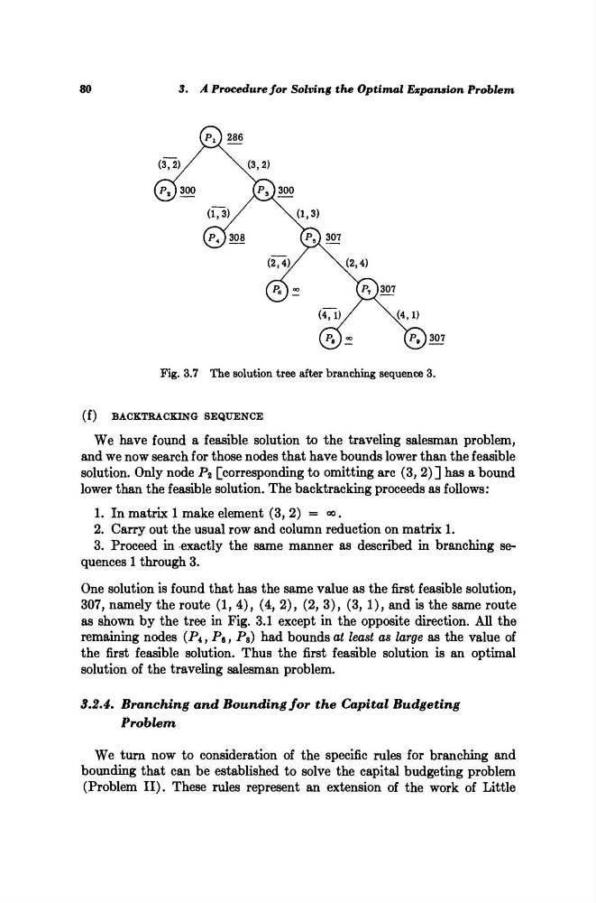
Fig. 3.7 The solution tree after branching sequence 3.
(f)
BACKTRACKING SEQUENCE
We have found a feasible solution to the traveling salesman problem,
and we now search for those nodes that have bounds lower than the feasible
solution. Only node P% [corresponding to omitting arc (3, 2) ] has a bound
lower than the feasible solution. The backtracking proceeds as follows:
1. In matrix 1 make element (3, 2) = <*>.
2. Carry out the usual row and column reduction on matrix 1.
3. Proceed in exactly the same manner as described in branching sequences 1 through 3.
One solution is found that has the same value as the first feasible solution,
307, namely the route (1, 4), (4, 2), (2, 3), (3, 1), and is the same route
as shown by the tree in Fig. 3.1 except in the opposite direction. All the
remaining nodes (PA , Pe, Ps) had bounds at least as large as the value of
the first feasible solution. Thus the first feasible solution is an optimal
solution of the traveling salesman problem.
3.2.4. Branching
and Bounding for the Capital
Budgeting
Problem
We turn now to consideration of the specific rules for branching and
bounding that can be established to solve the capital budgeting problem
(Problem II). These rules represent an extension of the work of Little
3. A Procedure for Solving the Optimal Expansion
Problem
Fig. 3.7 The solution tree after branching sequence 3.
(f)
BACKTRACKING SEQUENCE
We have found a feasible solution to the traveling salesman problem,
and we now search for those nodes that have bounds lower than the feasible
solution. Only node P% [corresponding to omitting arc (3, 2) ] has a bound
lower than the feasible solution. The backtracking proceeds as follows:
1. In matrix 1 make element (3, 2) = <*>.
2. Carry out the usual row and column reduction on matrix 1.
3. Proceed in exactly the same manner as described in branching sequences 1 through 3.
One solution is found that has the same value as the first feasible solution,
307, namely the route (1, 4), (4, 2), (2, 3), (3, 1), and is the same route
as shown by the tree in Fig. 3.1 except in the opposite direction. All the
remaining nodes (PA , Pe, Ps) had bounds at least as large as the value of
the first feasible solution. Thus the first feasible solution is an optimal
solution of the traveling salesman problem.
3.2.4. Branching
and Bounding for the Capital
Budgeting
Problem
We turn now to consideration of the specific rules for branching and
bounding that can be established to solve the capital budgeting problem
(Problem II). These rules represent an extension of the work of Little