

20
1.
Introduction
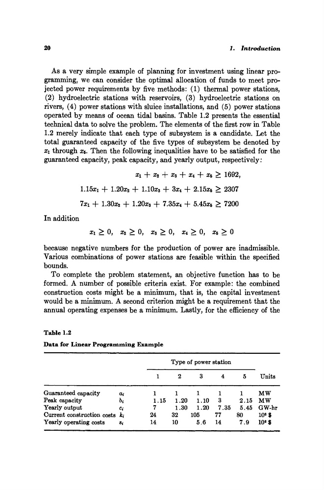
As a very simple example of planning for investment using linear programming, we can consider the optimal allocation of funds to meet projected power requirements by five methods: (1) thermal power stations,
(2) hydroelectric stations with reservoirs, (3) hydroelectric stations on
rivers, (4) power stations with sluice installations, and (5) power stations
operated by means of ocean tidal basins. Table 1.2 presents the essential
technical data to solve the problem. The elements of the first row in Table
1.2 merely indicate that each type of subsystem is a candidate. Let the
total guaranteed capacity of the five types of subsystem be denoted by
Xi through ft. Then the following inequalities have to be satisfied for the
guaranteed capacity, peak capacity, and yearly output, respectively:
ft + ft + ft + ft + ft > 1692,
1.15ft + 1.20ft + 1.10ft + 3ft + 2.15a* > 2307
7ft + 1.30ft + 1.20ft + 7.35ft + 5.45ft > 7200
In addition
ft > 0, ft > 0, ft > 0, ft > 0, ft > 0
because negative numbers for the production of power are inadmissible.
Various combinations of power stations are feasible within the specified
bounds.
To complete the problem statement, an objective function has to be
formed. A number of possible criteria exist. For example: the combined
construction costs might be a minimum, that is, the capital investment
would be a minimum. A second criterion might be a requirement that the
annual operating expenses be a minimum. Lastly, for the efficiency of the
Table 1.2
Data for Linear Programming Example
Type of power station
1
2
3
4
5
Units
Guaranteed capacityOf
1
1
1
1
1
MW
Peak capacity
b<
1.15
1.20
1.10
3
2.15 MW
Yearly output
Ci
7
1.30
1.20
7.35
5.45 GW-hr
Current construction costs hi
24
32
105
77
80
10" $
Yearly operating costs
Si
14
10
5.6
14
7.9
10«$
1.
Introduction
As a very simple example of planning for investment using linear programming, we can consider the optimal allocation of funds to meet projected power requirements by five methods: (1) thermal power stations,
(2) hydroelectric stations with reservoirs, (3) hydroelectric stations on
rivers, (4) power stations with sluice installations, and (5) power stations
operated by means of ocean tidal basins. Table 1.2 presents the essential
technical data to solve the problem. The elements of the first row in Table
1.2 merely indicate that each type of subsystem is a candidate. Let the
total guaranteed capacity of the five types of subsystem be denoted by
Xi through ft. Then the following inequalities have to be satisfied for the
guaranteed capacity, peak capacity, and yearly output, respectively:
ft + ft + ft + ft + ft > 1692,
1.15ft + 1.20ft + 1.10ft + 3ft + 2.15a* > 2307
7ft + 1.30ft + 1.20ft + 7.35ft + 5.45ft > 7200
In addition
ft > 0, ft > 0, ft > 0, ft > 0, ft > 0
because negative numbers for the production of power are inadmissible.
Various combinations of power stations are feasible within the specified
bounds.
To complete the problem statement, an objective function has to be
formed. A number of possible criteria exist. For example: the combined
construction costs might be a minimum, that is, the capital investment
would be a minimum. A second criterion might be a requirement that the
annual operating expenses be a minimum. Lastly, for the efficiency of the
Table 1.2
Data for Linear Programming Example
Type of power station
1
2
3
4
5
Units
Guaranteed capacityOf
1
1
1
1
1
MW
Peak capacity
b<
1.15
1.20
1.10
3
2.15 MW
Yearly output
Ci
7
1.30
1.20
7.35
5.45 GW-hr
Current construction costs hi
24
32
105
77
80
10" $
Yearly operating costs
Si
14
10
5.6
14
7.9
10«$