

BINARY RANDOM WALKS: ADDENDUM
65
(10)
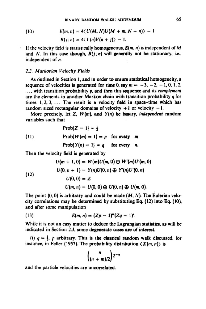
E(m, n ) = 4(L'(M, N ) U ( M + m, N + n ) ) - I
R ( / : n ) = 4(C'(lI)V(n + j)) - 1.
If the velocity field is statistically bomopeoue, E(m, n ) is independent of M
and N. In this case though, R(j; n) will generally not be stationary, i.e.,
independent of n.
2.2. Markooian Velocity Fields
As outlined in Section 1, and in order to ensure statbtical homogeneity, a
sequence of velocities is generated for time 0, ~loy M = -3, -2, - 1.0, 1.2,
. . . , with transition probability p, and then this sequence and its complement
are the elements in another Markov chain with transition probability q for
times 1.2, 3,. . . . The result is a velocity field in space-time which has
random sized rectangular domains of velocity -k 1 or velocity - 1.
More precisely, let 2, W(m), and Y(n) be W r y , independetrf random
variables such that
Prob(2 = I ) = f
(1 1)
Prob(W(m) = I} p . p for every m
Prob{Y(n) = I} = q for every n.
Then the velocity field is generated by
U(m + 1,O) = W(m)U(m, 0 ) g) W,(m)U'(m, 0 )
U(0, n + 1) = Y(n)U(O, n ) @ Y'(n)U'(O, n )
Lr(0,O) = z
U(m, n ) = U(0,O) @ U(0, n ) e qm, 0).
The point (0,O) is arbitrary and could be made (M, N) Tbe Eulerian velocity correlations may be determined by substituting Eq. (12) into Eq. (lo),
and after some manipulation
(13)
E(m, n ) = ( Z p - 1F(Zq - 1)".
While it is not an easy matter to deduce the Lagrangian statistics, as will be
indicated in Section 2.3, some degenerate cases me of intertst.
(i) q = 4. p arbitrary. This is the classical random walk discussed, for
instance, in Feller (1957). The probability distribution (X(m, n ) ) is
( ( n + L ) 2 - *
and the particle velocities are uncorrelated.
65
(10)
E(m, n ) = 4(L'(M, N ) U ( M + m, N + n ) ) - I
R ( / : n ) = 4(C'(lI)V(n + j)) - 1.
If the velocity field is statistically bomopeoue, E(m, n ) is independent of M
and N. In this case though, R(j; n) will generally not be stationary, i.e.,
independent of n.
2.2. Markooian Velocity Fields
As outlined in Section 1, and in order to ensure statbtical homogeneity, a
sequence of velocities is generated for time 0, ~loy M = -3, -2, - 1.0, 1.2,
. . . , with transition probability p, and then this sequence and its complement
are the elements in another Markov chain with transition probability q for
times 1.2, 3,. . . . The result is a velocity field in space-time which has
random sized rectangular domains of velocity -k 1 or velocity - 1.
More precisely, let 2, W(m), and Y(n) be W r y , independetrf random
variables such that
Prob(2 = I ) = f
(1 1)
Prob(W(m) = I} p . p for every m
Prob{Y(n) = I} = q for every n.
Then the velocity field is generated by
U(m + 1,O) = W(m)U(m, 0 ) g) W,(m)U'(m, 0 )
U(0, n + 1) = Y(n)U(O, n ) @ Y'(n)U'(O, n )
Lr(0,O) = z
U(m, n ) = U(0,O) @ U(0, n ) e qm, 0).
The point (0,O) is arbitrary and could be made (M, N) Tbe Eulerian velocity correlations may be determined by substituting Eq. (12) into Eq. (lo),
and after some manipulation
(13)
E(m, n ) = ( Z p - 1F(Zq - 1)".
While it is not an easy matter to deduce the Lagrangian statistics, as will be
indicated in Section 2.3, some degenerate cases me of intertst.
(i) q = 4. p arbitrary. This is the classical random walk discussed, for
instance, in Feller (1957). The probability distribution (X(m, n ) ) is
( ( n + L ) 2 - *
and the particle velocities are uncorrelated.