

O*€
0.E
sw 0.4
0.2
0
-0.2
Su - 0 . 4
-0.6
-0.8
-
TURBLJLENCE IN AN INTERNAL BOUNDARY LAYER
269
0
-1
n
0
A
-
A
0
-
A
- - 2 S"W
-3
-4
I
0 -
-
1.0
2.0
3.0
Z / 6 i
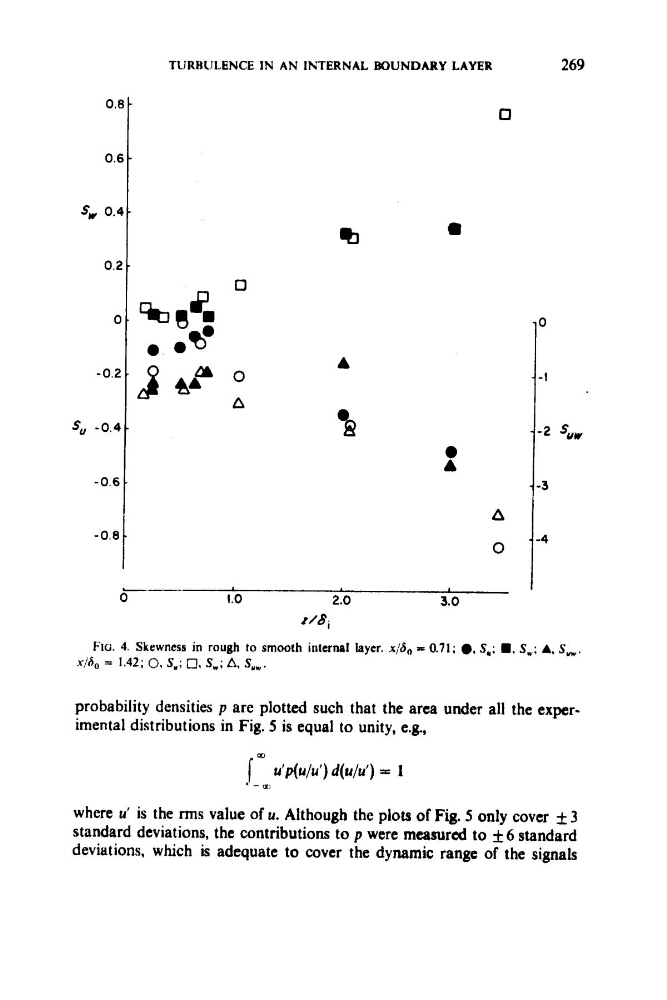
Flu. 4. Skewness in rough to smooth internal layer. X:So = 0.71; 0, S,; ., S, ; A, S, .
.Y/ho 3 1.42; 0. S,; 0. S,; A, Suw.
probability densities p are plotted such that the area under all the experimental distributions in Fig. 5 is equal to unity, e.g.,
(0
1 u'p(u/u')d(u/u') = 1
. _
where u' is the rms value of u. Although the plots of Fig. 5 only cover f 3
standard deviations, the contributions to p were measured to I t 6 standard
deviations, which is adequate to cover the dynamic range of the signals
0.E
sw 0.4
0.2
0
-0.2
Su - 0 . 4
-0.6
-0.8
-
TURBLJLENCE IN AN INTERNAL BOUNDARY LAYER
269
0
-1
n
0
A
-
A
0
-
A
- - 2 S"W
-3
-4
I
0 -
-
1.0
2.0
3.0
Z / 6 i
Flu. 4. Skewness in rough to smooth internal layer. X:So = 0.71; 0, S,; ., S, ; A, S, .
.Y/ho 3 1.42; 0. S,; 0. S,; A, Suw.
probability densities p are plotted such that the area under all the experimental distributions in Fig. 5 is equal to unity, e.g.,
(0
1 u'p(u/u')d(u/u') = 1
. _
where u' is the rms value of u. Although the plots of Fig. 5 only cover f 3
standard deviations, the contributions to p were measured to I t 6 standard
deviations, which is adequate to cover the dynamic range of the signals