

NlIMERICAL COMPUTATION OF TURBULENT SHEAR FLOWS
233
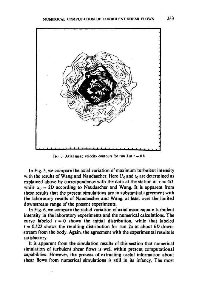
Flci. 3. Axial mean velocity contours for run 3 at t = 0.8.
In Fig. 5, we compare the axial variation of maximum turbulent intensity
with the results of Wang and Naudascher. Here U, and to are determined as
explained above by correspondence with the data at the station at x = 40,
while xo = 2D according to Naudascher and Wang. It is apparent from
these results that the present simulations are in substantial agreement with
the laboratory results of Naudascher and Wan& at least over the limited
downstream range of the present experiments.
In Fig. 6, we compare the radial variation of axial mean-square turbulent
intensity in the laboratory experiments and the numerical calculations. The
curve labeled t = 0 shows the initial distribution, while that labeled
t = 0.522 shows the resulting distribution for run 2a at about 6 0 downstream from the body. Again, the agreement with the experimental results is
satisfactory.
It is apparent from the simulation results of this section that numerical
simulation of turbulent shear flows is well within present computational
capabilities. However, the process of extracting useful information about
shear flows from numerical simulations is still in its infancy. The most
233
Flci. 3. Axial mean velocity contours for run 3 at t = 0.8.
In Fig. 5, we compare the axial variation of maximum turbulent intensity
with the results of Wang and Naudascher. Here U, and to are determined as
explained above by correspondence with the data at the station at x = 40,
while xo = 2D according to Naudascher and Wang. It is apparent from
these results that the present simulations are in substantial agreement with
the laboratory results of Naudascher and Wan& at least over the limited
downstream range of the present experiments.
In Fig. 6, we compare the radial variation of axial mean-square turbulent
intensity in the laboratory experiments and the numerical calculations. The
curve labeled t = 0 shows the initial distribution, while that labeled
t = 0.522 shows the resulting distribution for run 2a at about 6 0 downstream from the body. Again, the agreement with the experimental results is
satisfactory.
It is apparent from the simulation results of this section that numerical
simulation of turbulent shear flows is well within present computational
capabilities. However, the process of extracting useful information about
shear flows from numerical simulations is still in its infancy. The most