

NUMERICAL COMPUTATION OF TURBULENT SHEAR FLOWS
229
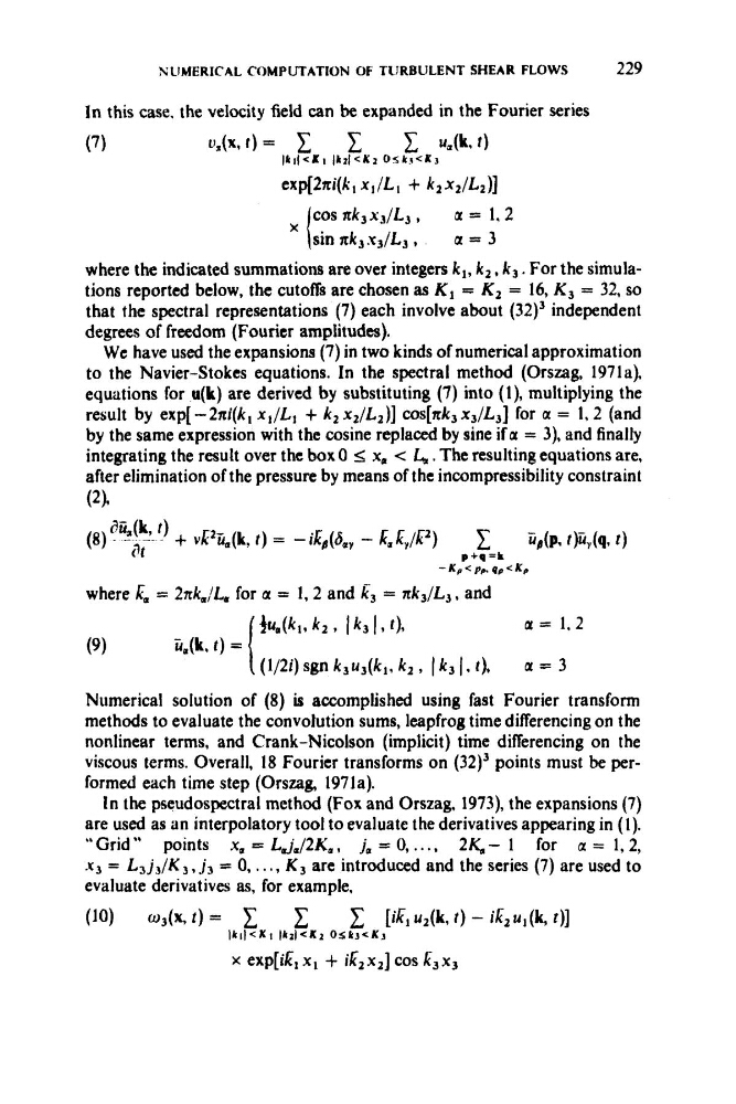
In this case. the velocity field can be expanded in the Fourier series
v,(x, I ) = c c c 4 k . I )
J k I ( < X i l k l l < K z O S k i < K 3
(7)
expE2ni(kl xl/L, + k2x2/L2)]
a = 3
cos x k 3 x 3 / L 3 , a = 1.2
.( sin ak3x3/L3 ,
where the indicated summations are over integers kl, k,, k 3 . For the simulations reported below, the cutoffs are chosen as K1 = K 2 = 16, K 3 = 32, so
that the spectral representations (7) each involve about (32)’ independent
degrees of freedom (Fourier amplitudes).
We have used the expansions (7) in two kinds of numerical approximation
to the Navier-Stokes equations. In the spectral method (Orszag, 1971a).
equations for u(k) are derived by substituting (7) into (l), multiplying the
result by exp[ -2ni(k, xl/Ll + k 2 x 2 / L , ) ] cos[nk3x3/L3] for a = 1,2 (and
by the same expression with the cosine replaced by sine if a = 3), and finally
integrating the result over the box 0 5 x, < L, . The resulting equations are,
after elimination of the pressure by means of the incompressibility constraint
- K P < P P . Q P < K P
where Lu = ZnkJL, for a = 1,2 and k3 = xkJ/L3, and
(9)
t,(k, t ) =
Numerical solution of (8) is accomplished using fast Fourier transform
methods to evaluate the convolution sums, leapfrog time differencing on the
nonlinear terms, and Crank-Nicolson (implicit) time differencing on the
viscous terms. Overall, 18 Fourier transforms on (32)3 points must be performed each time step (Orszag, 1971a).
In the pseudospectral method (Fox and Orszag. 1973), the expansions (7)
are used as an interpolatory tool to evaluate the derivatives appearing in (1).
“Grid” points x, = Laj,/2K,, j, = 0, .. .. 2&- 1 for a = 1, 2,
x3 = L3 j , / K ,, j , = 0, . . . , K 3 are introduced and the series (7) are used to
evaluate derivatives as, for example,
4um(kl, k 2 9 I k3 I , t).
a = 1.2
1 (1/2i) sgn k3u3(k,, k2 , I k3 1, I). a = 3
x exp[iKl x l + i/i2x2] cos k3x3
229
In this case. the velocity field can be expanded in the Fourier series
v,(x, I ) = c c c 4 k . I )
J k I ( < X i l k l l < K z O S k i < K 3
(7)
expE2ni(kl xl/L, + k2x2/L2)]
a = 3
cos x k 3 x 3 / L 3 , a = 1.2
.( sin ak3x3/L3 ,
where the indicated summations are over integers kl, k,, k 3 . For the simulations reported below, the cutoffs are chosen as K1 = K 2 = 16, K 3 = 32, so
that the spectral representations (7) each involve about (32)’ independent
degrees of freedom (Fourier amplitudes).
We have used the expansions (7) in two kinds of numerical approximation
to the Navier-Stokes equations. In the spectral method (Orszag, 1971a).
equations for u(k) are derived by substituting (7) into (l), multiplying the
result by exp[ -2ni(k, xl/Ll + k 2 x 2 / L , ) ] cos[nk3x3/L3] for a = 1,2 (and
by the same expression with the cosine replaced by sine if a = 3), and finally
integrating the result over the box 0 5 x, < L, . The resulting equations are,
after elimination of the pressure by means of the incompressibility constraint
- K P < P P . Q P < K P
where Lu = ZnkJL, for a = 1,2 and k3 = xkJ/L3, and
(9)
t,(k, t ) =
Numerical solution of (8) is accomplished using fast Fourier transform
methods to evaluate the convolution sums, leapfrog time differencing on the
nonlinear terms, and Crank-Nicolson (implicit) time differencing on the
viscous terms. Overall, 18 Fourier transforms on (32)3 points must be performed each time step (Orszag, 1971a).
In the pseudospectral method (Fox and Orszag. 1973), the expansions (7)
are used as an interpolatory tool to evaluate the derivatives appearing in (1).
“Grid” points x, = Laj,/2K,, j, = 0, .. .. 2&- 1 for a = 1, 2,
x3 = L3 j , / K ,, j , = 0, . . . , K 3 are introduced and the series (7) are used to
evaluate derivatives as, for example,
4um(kl, k 2 9 I k3 I , t).
a = 1.2
1 (1/2i) sgn k3u3(k,, k2 , I k3 1, I). a = 3
x exp[iKl x l + i/i2x2] cos k3x3