

1 R4
1. I.. I.IIMI.EY A h 1 1 H. YHAJEH-NOI’RI
I
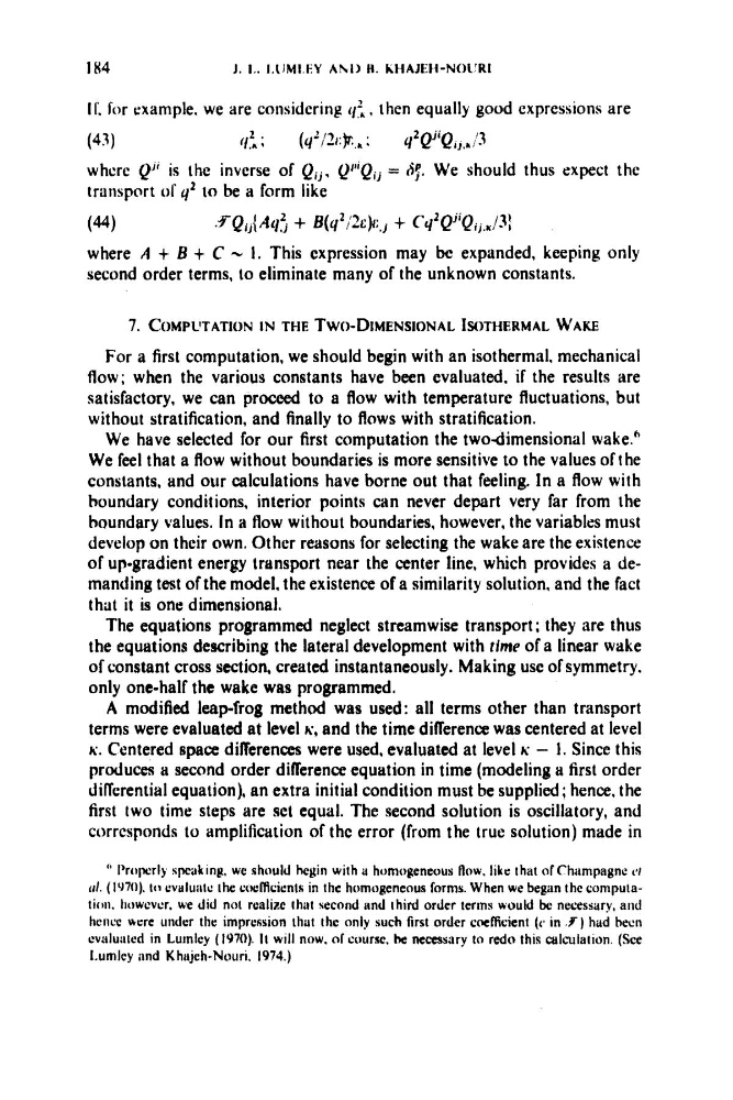
C for cxample. we are considering I I ? ~ , then equally good expressions are
(I.&, 2 .
(y’,”~:p’.,~ ;
y2Qj‘Qij,,/3
(43)
whcrc P’‘ is the inverse of Q i j . Q”iQij = iip. We should thus expect the
transport or 4’ to be a form like
(44)
.FQij(Aq: + B(y2/’2~jl:.j + C$QJiQijJ3]
where A + B + C - 1. This expression may be expanded, keeping only
second order terms, to eliminate many of the unknown constants.
7. COMPL~TATION I N THE TWO-DIMENSIONAL ISOTHERMAL WAKE
For a first computation, we should begin with an isothermal, mechanical
flow; when the various constants have been evaluated. if the results are
satisfactory, we can proceed to a flow with temperature fluctuations, but
without stratification, and finally to flows with stratification.
We have selected for our first computation the twodimensional wake.’
We feel that a flow without boundaries is more sensitive to the values of the
constants, and our calculations have borne out that feeling. In a flow with
boundary conditions, interior points can never depart very far from the
boundary values. In a flow without boundaries, however, the variables must
develop on thcir own. Other reasons for selecting the wake are the existence
of up-gradient energy transport near the center line, which provides a demanding test of the model, the existence of a similarity solution. and the fact
that it is one dimensional.
The equations programmed neglect streamwise transport; they are thus
the equations describing the lateral development with rime of a linear wake
of constant cross section, created instantaneously. Making use of symmetry.
only one-half the wake was programmed.
A modified leapfrog method was used: all terms other than transport
terms were evaluated at level K, and the time difference was centered at level
K. Centered space differences were used, evaluated at level K - 1. Since this
produces B second order difference equation in time (modeling a first order
differential equation), an extra initial condition must be supplied; hence, the
first two time steps are set equal. The second solution is oscillatory, and
corresponds to amplification of thc error (from the true solution) made in
” I’roperly spakinp. we should hcyin with a homogeneous flow. like that of Chiirnpagnc c’i
ti/. ( I1J70). 111 uvtiluntc the cocfficientr in the homogencouc forms. When we began the cornpulation. Iiowcvcr. we did not redim that second and ihird order terms would be necessary, atid
hciicc were under the! impression that the only such first order coefficient (c in Y ) had becn
cvcrluatcd in Lurnlcy ( 1970). It will now, or course, k necessary to redo this wldation. (See
I.urnley and Khujeh-Nouri. 1974.)
1. I.. I.IIMI.EY A h 1 1 H. YHAJEH-NOI’RI
I
C for cxample. we are considering I I ? ~ , then equally good expressions are
(I.&, 2 .
(y’,”~:p’.,~ ;
y2Qj‘Qij,,/3
(43)
whcrc P’‘ is the inverse of Q i j . Q”iQij = iip. We should thus expect the
transport or 4’ to be a form like
(44)
.FQij(Aq: + B(y2/’2~jl:.j + C$QJiQijJ3]
where A + B + C - 1. This expression may be expanded, keeping only
second order terms, to eliminate many of the unknown constants.
7. COMPL~TATION I N THE TWO-DIMENSIONAL ISOTHERMAL WAKE
For a first computation, we should begin with an isothermal, mechanical
flow; when the various constants have been evaluated. if the results are
satisfactory, we can proceed to a flow with temperature fluctuations, but
without stratification, and finally to flows with stratification.
We have selected for our first computation the twodimensional wake.’
We feel that a flow without boundaries is more sensitive to the values of the
constants, and our calculations have borne out that feeling. In a flow with
boundary conditions, interior points can never depart very far from the
boundary values. In a flow without boundaries, however, the variables must
develop on thcir own. Other reasons for selecting the wake are the existence
of up-gradient energy transport near the center line, which provides a demanding test of the model, the existence of a similarity solution. and the fact
that it is one dimensional.
The equations programmed neglect streamwise transport; they are thus
the equations describing the lateral development with rime of a linear wake
of constant cross section, created instantaneously. Making use of symmetry.
only one-half the wake was programmed.
A modified leapfrog method was used: all terms other than transport
terms were evaluated at level K, and the time difference was centered at level
K. Centered space differences were used, evaluated at level K - 1. Since this
produces B second order difference equation in time (modeling a first order
differential equation), an extra initial condition must be supplied; hence, the
first two time steps are set equal. The second solution is oscillatory, and
corresponds to amplification of thc error (from the true solution) made in
” I’roperly spakinp. we should hcyin with a homogeneous flow. like that of Chiirnpagnc c’i
ti/. ( I1J70). 111 uvtiluntc the cocfficientr in the homogencouc forms. When we began the cornpulation. Iiowcvcr. we did not redim that second and ihird order terms would be necessary, atid
hciicc were under the! impression that the only such first order coefficient (c in Y ) had becn
cvcrluatcd in Lurnlcy ( 1970). It will now, or course, k necessary to redo this wldation. (See
I.urnley and Khujeh-Nouri. 1974.)