

I x2
I - ~ i ~ i i l l y .
we may ;ippIy thc sallic proccdurc to ohtiiili the forms for thc
light-hiilld sides of ( 1 ) and (7). The right-hand side of (I 1 t11ust hc ii sciilar
fiinctional of the s u m variiibles HS (31). Complete lo teriiis of third order.
thc right-hand side of (I) is
(36)
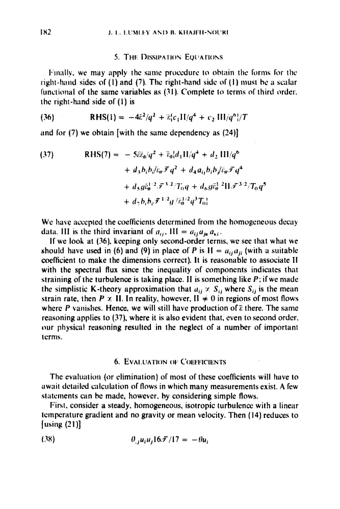
RHS(1) = -4E2/y2 + E(o,II/yJ + c2 IlI/qhj/T
and for (7) we obtain [with the same dependency as (74)]
We have iicccpted the coefficients determined from the homogeneous decay
data. 111 is the third invariant of q i , 111 = ( i i j u j N a r i .
If we look at (36). keeping only second-order ternis, we sec that what we
should have used in (6) and (9) in place of P is I1 = u i j ( I j i (with a suitable
coefficient to make the dimensions correct). It is reasonable to associate I I
with the spectral flux since the inequality of components indicates that
straining of the turbulence is taking place. I1 is something like P ; if we made
the simplistic K-theory tipproximittion that
x. S i i where Sij is the mean
strain rate, then P x 11. In reality, however, 11 i 0 in regions of most flows
whcrc P vanishes. Hence, we will still have production ofZ there. The same
reitsoning applies to (37). where it is also evident that. even to second order,
our physical reasoning resulted in the neglect of a number of important
tcrms.
6. EVAI.CIAW)N 01, COEFFICIENTS
The evtillliltic)tl (or elimination) of most of these coefficients will have to
awaii detailcd c:ilculation of flows in which many measurements exist. A few
sliitcinents citn be made. however, by considering simple flows.
First, consider a steady, homogeneous, isotropic turbulence with a linear
lempcrature gradient and no gravity or mean velocity. Then (14) reduces to
[using (2111
(:IN)
O~j~~it~I6.Y/17 = -OU,
I - ~ i ~ i i l l y .
we may ;ippIy thc sallic proccdurc to ohtiiili the forms for thc
light-hiilld sides of ( 1 ) and (7). The right-hand side of (I 1 t11ust hc ii sciilar
fiinctional of the s u m variiibles HS (31). Complete lo teriiis of third order.
thc right-hand side of (I) is
(36)
RHS(1) = -4E2/y2 + E(o,II/yJ + c2 IlI/qhj/T
and for (7) we obtain [with the same dependency as (74)]
We have iicccpted the coefficients determined from the homogeneous decay
data. 111 is the third invariant of q i , 111 = ( i i j u j N a r i .
If we look at (36). keeping only second-order ternis, we sec that what we
should have used in (6) and (9) in place of P is I1 = u i j ( I j i (with a suitable
coefficient to make the dimensions correct). It is reasonable to associate I I
with the spectral flux since the inequality of components indicates that
straining of the turbulence is taking place. I1 is something like P ; if we made
the simplistic K-theory tipproximittion that
x. S i i where Sij is the mean
strain rate, then P x 11. In reality, however, 11 i 0 in regions of most flows
whcrc P vanishes. Hence, we will still have production ofZ there. The same
reitsoning applies to (37). where it is also evident that. even to second order,
our physical reasoning resulted in the neglect of a number of important
tcrms.
6. EVAI.CIAW)N 01, COEFFICIENTS
The evtillliltic)tl (or elimination) of most of these coefficients will have to
awaii detailcd c:ilculation of flows in which many measurements exist. A few
sliitcinents citn be made. however, by considering simple flows.
First, consider a steady, homogeneous, isotropic turbulence with a linear
lempcrature gradient and no gravity or mean velocity. Then (14) reduces to
[using (2111
(:IN)
O~j~~it~I6.Y/17 = -OU,