

The computation procedure involved the iisc of a fourth-order Arakii\h.it
finite difference scheinc and a leapfrog type tinie differencing scheme. The
Poisson equation was solved bq use of Fourier transform. in porticular. the
fast Fourier transform algorithm. Application of this was possible ill
the axial ilnd transverse directions because of the periodicity of the boundary conditions and effectively implies an exact solution at the mesh points
for each vertical level.
3.1.2. Etrlcriait Resrrlrs. Computations were performed for all details o f
the Eulerian field and various output information was obtained by direct
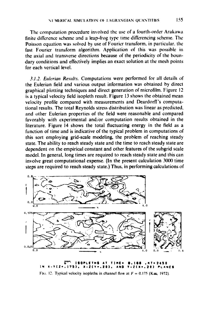
graphical plotting techniques and direct generation of microfilm. Figure I2
is a typical velocity field isopleth result. Figure 13 shows the obtained mean
velocity profile compared with measurements and Deardorff's computational results. The total Reynolds stress distribution was linear as predicted,
and other Eulerian properties of the field were reasonable and compared
favorably with experimental and/or computation results obtained in the
literature. Figure 14 shows the total fiuctuating energy in the field as a
function of time and is indicative of the typical problem in computations of
this sort employing grid-scale modeling, the problem of reaching steady
state. The ability to reach steady state and the time to reach steady state are
dependent on the empirical constant and other features of the subgrid scale
model. In general, long times are required to reach steady state and this can
involve great computational expense. (In the present calculation 3ooO time
steps are required to reach steady state.) Thus. in performing calculations of
,
I
0 . 0 2 5
4.6
-.I
0 . 0
0.0
__ \ 0 . M
finite difference scheinc and a leapfrog type tinie differencing scheme. The
Poisson equation was solved bq use of Fourier transform. in porticular. the
fast Fourier transform algorithm. Application of this was possible ill
the axial ilnd transverse directions because of the periodicity of the boundary conditions and effectively implies an exact solution at the mesh points
for each vertical level.
3.1.2. Etrlcriait Resrrlrs. Computations were performed for all details o f
the Eulerian field and various output information was obtained by direct
graphical plotting techniques and direct generation of microfilm. Figure I2
is a typical velocity field isopleth result. Figure 13 shows the obtained mean
velocity profile compared with measurements and Deardorff's computational results. The total Reynolds stress distribution was linear as predicted,
and other Eulerian properties of the field were reasonable and compared
favorably with experimental and/or computation results obtained in the
literature. Figure 14 shows the total fiuctuating energy in the field as a
function of time and is indicative of the typical problem in computations of
this sort employing grid-scale modeling, the problem of reaching steady
state. The ability to reach steady state and the time to reach steady state are
dependent on the empirical constant and other features of the subgrid scale
model. In general, long times are required to reach steady state and this can
involve great computational expense. (In the present calculation 3ooO time
steps are required to reach steady state.) Thus. in performing calculations of
,
I
0 . 0 2 5
4.6
-.I
0 . 0
0.0
__ \ 0 . M