

landscapes. The only exception was the ASTER subscene for the downtown
landscape. It thus implies that the residential and downtown textural complexity
recorded by the three image types was mostly similar when resampled to the 120 m
pixel size. This corresponds to the finding from Figures 12.8b,c. When only the
resampled images were taken into account, those more distinct from others were both
observed to be the 120 m level for the ETM+ data regardless of their dominant
landscape as each displayed a total difference of 1.0. However, for image subscenes
from the ASTER and IKONOS data, the aggregation scales that were mostly different
from others were the 60 m for the residential landscape (total difference values of
1.989 and 1.182) but 30 m for the downtown landscape (total difference values of
1.702 and 1.252). As a result, for all three image types used to represent the two urban
landscapes, aggregation levels of 120, 60, and 30 m could generate image surfaces
that were more distinct from those from other aggregation levels (Figure 12.8a).
12.4.4 Fractal Analysis for Temporal Change Characterization
In order to assess the utility of FD analysis for characterizing the temporal change of
the landscape in the study area, all four Landsat images, including three TM and one
ETM+, were applied since together they represented a complete time series of 25
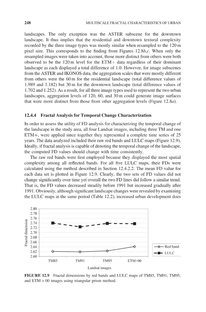
years. The data analyzed included their raw red bands and LULC maps (Figure 12.9).
Ideally, if fractal analysis is capable of denoting the temporal change of the landscape,
the computed FD values should change with time consistently.
The raw red bands were first employed because they displayed the most spatial
complexity among all reflected bands. For all five LULC maps, their FDs were
calculated using the method described in Section 12.4.2.2. The mean FD value for
each data set is plotted in Figure 12.9. Clearly, the two sets of FD values did not
change significantly over time yet overall the two FD lines did follow a similar trend.
That is, the FD values decreased steadily before 1991 but increased gradually after
1991. Obviously, although significant landscape changes were revealed by examining
the LULC maps at the same period (Table 12.2), increased urban development does
FIGURE 12.9 Fractal dimensions by red bands and LULC maps of TM85, TM91, TM95,
and ETM + 00 images using triangular prism method.
248
MULTISCALE FRACTAL CHARACTERISTICS OF URBAN
landscape. It thus implies that the residential and downtown textural complexity
recorded by the three image types was mostly similar when resampled to the 120 m
pixel size. This corresponds to the finding from Figures 12.8b,c. When only the
resampled images were taken into account, those more distinct from others were both
observed to be the 120 m level for the ETM+ data regardless of their dominant
landscape as each displayed a total difference of 1.0. However, for image subscenes
from the ASTER and IKONOS data, the aggregation scales that were mostly different
from others were the 60 m for the residential landscape (total difference values of
1.989 and 1.182) but 30 m for the downtown landscape (total difference values of
1.702 and 1.252). As a result, for all three image types used to represent the two urban
landscapes, aggregation levels of 120, 60, and 30 m could generate image surfaces
that were more distinct from those from other aggregation levels (Figure 12.8a).
12.4.4 Fractal Analysis for Temporal Change Characterization
In order to assess the utility of FD analysis for characterizing the temporal change of
the landscape in the study area, all four Landsat images, including three TM and one
ETM+, were applied since together they represented a complete time series of 25
years. The data analyzed included their raw red bands and LULC maps (Figure 12.9).
Ideally, if fractal analysis is capable of denoting the temporal change of the landscape,
the computed FD values should change with time consistently.
The raw red bands were first employed because they displayed the most spatial
complexity among all reflected bands. For all five LULC maps, their FDs were
calculated using the method described in Section 12.4.2.2. The mean FD value for
each data set is plotted in Figure 12.9. Clearly, the two sets of FD values did not
change significantly over time yet overall the two FD lines did follow a similar trend.
That is, the FD values decreased steadily before 1991 but increased gradually after
1991. Obviously, although significant landscape changes were revealed by examining
the LULC maps at the same period (Table 12.2), increased urban development does
FIGURE 12.9 Fractal dimensions by red bands and LULC maps of TM85, TM91, TM95,
and ETM + 00 images using triangular prism method.
248
MULTISCALE FRACTAL CHARACTERISTICS OF URBAN