

8.2.3.1 Gray-Level Blob Delineation Operationalizing this concept of SS persistence is not trivial and involves a number of components, which we will only briefly
describe. For more detailed information see Lindeberg (1994) and Hay et al. (2002a).
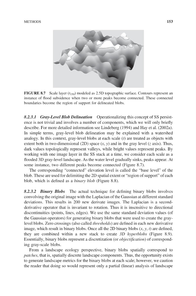
In simple terms, gray-level blob delineation may be explained with a watershed
analogy. In this context, gray-level blobs at each scale (t) are treated as objects with
extent both in two-dimensional (2D) space (x, y) and in the gray level (z axis). Thus,
dark values topologically represent valleys, while bright values represent peaks. By
working with one image layer in the SS stack at a time, we consider each scale as a
flooded 3D gray-level landscape. As the water level gradually sinks, peaks appear. At
some instance, two different peaks become connected (Figure 8.7).
The corresponding “connected” elevation level is called the “base level” of the
blob. These are used for delimiting the 2D spatial extent or “region of support” of each
blob, which is defined as a binary blob (Figure 8.8).
8.2.3.2 Binary Blobs The actual technique for defining binary blobs involves
convolving the original image with the Laplacian of the Gaussian at different standard
deviations. This results in 200 new derivate images. The Laplacian is a secondderivative operator that is invariant to rotation. Thus it is insensitive to directional
discontinuities (points, lines, edges). We use the same standard deviation values (of
the Gaussian operators) for generating binary blobs that were used to create the graylevel blobs. Zero crossings (also called thresholds) are defined in each new derivative
image, which result in binary blobs. Once all the 2D binary blobs (x, y, t) are defined,
they are combined within a new stack to create 3D hyperblobs (Figure 8.9).
Essentially, binary blobs represent a discretization (or objectification) of corresponding gray-scale blobs.
From a landscape ecology perspective, binary blobs spatially correspond to
patches, that is, spatially discrete landscape components. Thus, the opportunity exists
to generate landscape metrics for the binary blobs at each scale; however, we caution
the reader that doing so would represent only a partial (linear) analysis of landscape
FIGURE 8.7 Scale layer (t 150 ) modeled as 2.5D topographic surface. Contours represent an
instance of flood subsidence when two or more peaks become connected. These connected
boundaries become the region of support for delineated blobs.
METHODS
153
describe. For more detailed information see Lindeberg (1994) and Hay et al. (2002a).
In simple terms, gray-level blob delineation may be explained with a watershed
analogy. In this context, gray-level blobs at each scale (t) are treated as objects with
extent both in two-dimensional (2D) space (x, y) and in the gray level (z axis). Thus,
dark values topologically represent valleys, while bright values represent peaks. By
working with one image layer in the SS stack at a time, we consider each scale as a
flooded 3D gray-level landscape. As the water level gradually sinks, peaks appear. At
some instance, two different peaks become connected (Figure 8.7).
The corresponding “connected” elevation level is called the “base level” of the
blob. These are used for delimiting the 2D spatial extent or “region of support” of each
blob, which is defined as a binary blob (Figure 8.8).
8.2.3.2 Binary Blobs The actual technique for defining binary blobs involves
convolving the original image with the Laplacian of the Gaussian at different standard
deviations. This results in 200 new derivate images. The Laplacian is a secondderivative operator that is invariant to rotation. Thus it is insensitive to directional
discontinuities (points, lines, edges). We use the same standard deviation values (of
the Gaussian operators) for generating binary blobs that were used to create the graylevel blobs. Zero crossings (also called thresholds) are defined in each new derivative
image, which result in binary blobs. Once all the 2D binary blobs (x, y, t) are defined,
they are combined within a new stack to create 3D hyperblobs (Figure 8.9).
Essentially, binary blobs represent a discretization (or objectification) of corresponding gray-scale blobs.
From a landscape ecology perspective, binary blobs spatially correspond to
patches, that is, spatially discrete landscape components. Thus, the opportunity exists
to generate landscape metrics for the binary blobs at each scale; however, we caution
the reader that doing so would represent only a partial (linear) analysis of landscape
FIGURE 8.7 Scale layer (t 150 ) modeled as 2.5D topographic surface. Contours represent an
instance of flood subsidence when two or more peaks become connected. These connected
boundaries become the region of support for delineated blobs.
METHODS
153