

The reason might be due to large sampling distances (1–3 km) of the used permanent
and temporary plots.
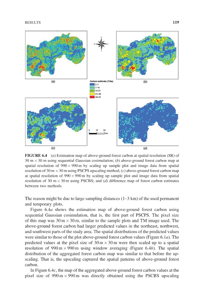
Figure 6.4a shows the estimation map of above-ground forest carbon using
sequential Gaussian cosimulation, that is, the first part of PSCPS. The pixel size
of this map was 30 m ´ 30 m, similar to the sample plots and TM image used. The
above-ground forest carbon had larger predicted values in the northeast, northwest,
and southwest parts of the study area. The spatial distributions of the predicted values
were similar to those of the plot above-ground forest carbon values (Figure 6.1a). The
predicted values at the pixel size of 30 m ´ 30 m were then scaled up to a spatial
resolution of 990 m ´ 990 m using window averaging (Figure 6.4b). The spatial
distribution of the aggregated forest carbon map was similar to that before the upscaling. That is, the upscaling captured the spatial patterns of above-ground forest
carbon.
In Figure 6.4c, the map of the aggregated above-ground forest carbon values at the
pixel size of 990 m ´ 990 m was directly obtained using the PSCBS upscaling
FIGURE 6.4 (a) Estimation map of above-ground forest carbon at spatial resolution (SR) of
30 m ´ 30 m using sequential Gaussian cosimulation; (b) above-ground forest carbon map at
spatial resolution of 990 ´ 990 m by scaling up sample plot and image data from spatial
resolution of 30 m ´ 30 m using PSCPS upscaling method; (c) above-ground forest carbon map
at spatial resolution of 990 ´ 990 m by scaling up sample plot and image data from spatial
resolution of 30 m ´ 30 m using PSCBS; and (d) difference map of forest carbon estimates
between two methods.
RESULTS
119
and temporary plots.
Figure 6.4a shows the estimation map of above-ground forest carbon using
sequential Gaussian cosimulation, that is, the first part of PSCPS. The pixel size
of this map was 30 m ´ 30 m, similar to the sample plots and TM image used. The
above-ground forest carbon had larger predicted values in the northeast, northwest,
and southwest parts of the study area. The spatial distributions of the predicted values
were similar to those of the plot above-ground forest carbon values (Figure 6.1a). The
predicted values at the pixel size of 30 m ´ 30 m were then scaled up to a spatial
resolution of 990 m ´ 990 m using window averaging (Figure 6.4b). The spatial
distribution of the aggregated forest carbon map was similar to that before the upscaling. That is, the upscaling captured the spatial patterns of above-ground forest
carbon.
In Figure 6.4c, the map of the aggregated above-ground forest carbon values at the
pixel size of 990 m ´ 990 m was directly obtained using the PSCBS upscaling
FIGURE 6.4 (a) Estimation map of above-ground forest carbon at spatial resolution (SR) of
30 m ´ 30 m using sequential Gaussian cosimulation; (b) above-ground forest carbon map at
spatial resolution of 990 ´ 990 m by scaling up sample plot and image data from spatial
resolution of 30 m ´ 30 m using PSCPS upscaling method; (c) above-ground forest carbon map
at spatial resolution of 990 ´ 990 m by scaling up sample plot and image data from spatial
resolution of 30 m ´ 30 m using PSCBS; and (d) difference map of forest carbon estimates
between two methods.
RESULTS
119