

forest carbon by weighting the sample plot data, collocated image data, and previous
estimates if any within the given neighborhood. The weights vary depending on the
spatial variability determined by the spatial configuration of the data (Goovaerts,
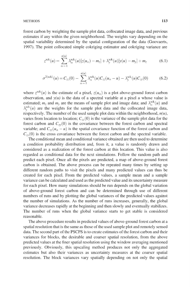
1997). The point collocated simple cokriging estimator and cokriging variance are
z
sck
u =
X n u
a = 1
l
sck
a uz u a − m z + l
sck
y uy u − m y + m z
(6.1)
s
2 sck
u = C zz 0 −
X n u
a = 1
l
sck
a uC zz u a − u − l
sck
y uC zy 0
(6.2)
where z
sck
u is the estimate of a pixel, z u a is a plot above-ground forest carbon
observation, and y(u) is the data of a spectral variable at a pixel u whose value is
estimated; m z and m y are the means of sample plot and image data; and l
sck
a u and
l
sck
y u are the weights for the sample plot data and the collocated image data,
respectively. The number of the used sample plot data within the neighborhood, n(u),
varies from location to location; C zz 0 is the variance of the sample plot data for the
forest carbon and C zy 0 is the covariance between the forest carbon and spectral
variable; and C zz u a − u is the spatial covariance function of the forest carbon and
C zy 0 is the cross covariance between the forest carbon and the spectral variable.
The conditional mean and conditional variance obtained are then used to determine
a condition probability distribution and, from it, a value is randomly drawn and
considered as a realization of the forest carbon at this location. This value is also
regarded as conditional data for the next simulations. Follow the random path and
predict each pixel. Once all the pixels are predicted, a map of above-ground forest
carbon is obtained. The above process can be repeated many times by setting up
different random paths to visit the pixels and many predicted values can thus be
created for each pixel. From the predicted values, a sample mean and a sample
variance can be calculated and used as the predicted value and its uncertainty measure
for each pixel. How many simulations should be run depends on the global variation
of above-ground forest carbon and can be determined through use of different
numbers of runs and by plotting the global variances of the predicted values against
the number of simulations. As the number of runs increases, generally, the global
variance decreases rapidly at the beginning and then slowly and eventually stabilizes.
The number of runs when the global variance starts to get stable is considered
reasonable.
The above procedure results in predicted values of above-ground forest carbon at a
spatial resolution that is the same as those of the used sample plot and remotely sensed
data. The second part of the PSCPS is to create estimates of the forest carbon and their
variances for blocks, the desirable and coarser spatial resolution, from the above
predicted values at the finer spatial resolution using the window averaging mentioned
previously. Obviously, this upscaling method produces not only the aggregated
estimates but also their variances as uncertainty measures at the coarser spatial
resolution. The block variances vary spatially depending on not only the spatial
METHODS
113
estimates if any within the given neighborhood. The weights vary depending on the
spatial variability determined by the spatial configuration of the data (Goovaerts,
1997). The point collocated simple cokriging estimator and cokriging variance are
z
sck
u =
X n u
a = 1
l
sck
a uz u a − m z + l
sck
y uy u − m y + m z
(6.1)
s
2 sck
u = C zz 0 −
X n u
a = 1
l
sck
a uC zz u a − u − l
sck
y uC zy 0
(6.2)
where z
sck
u is the estimate of a pixel, z u a is a plot above-ground forest carbon
observation, and y(u) is the data of a spectral variable at a pixel u whose value is
estimated; m z and m y are the means of sample plot and image data; and l
sck
a u and
l
sck
y u are the weights for the sample plot data and the collocated image data,
respectively. The number of the used sample plot data within the neighborhood, n(u),
varies from location to location; C zz 0 is the variance of the sample plot data for the
forest carbon and C zy 0 is the covariance between the forest carbon and spectral
variable; and C zz u a − u is the spatial covariance function of the forest carbon and
C zy 0 is the cross covariance between the forest carbon and the spectral variable.
The conditional mean and conditional variance obtained are then used to determine
a condition probability distribution and, from it, a value is randomly drawn and
considered as a realization of the forest carbon at this location. This value is also
regarded as conditional data for the next simulations. Follow the random path and
predict each pixel. Once all the pixels are predicted, a map of above-ground forest
carbon is obtained. The above process can be repeated many times by setting up
different random paths to visit the pixels and many predicted values can thus be
created for each pixel. From the predicted values, a sample mean and a sample
variance can be calculated and used as the predicted value and its uncertainty measure
for each pixel. How many simulations should be run depends on the global variation
of above-ground forest carbon and can be determined through use of different
numbers of runs and by plotting the global variances of the predicted values against
the number of simulations. As the number of runs increases, generally, the global
variance decreases rapidly at the beginning and then slowly and eventually stabilizes.
The number of runs when the global variance starts to get stable is considered
reasonable.
The above procedure results in predicted values of above-ground forest carbon at a
spatial resolution that is the same as those of the used sample plot and remotely sensed
data. The second part of the PSCPS is to create estimates of the forest carbon and their
variances for blocks, the desirable and coarser spatial resolution, from the above
predicted values at the finer spatial resolution using the window averaging mentioned
previously. Obviously, this upscaling method produces not only the aggregated
estimates but also their variances as uncertainty measures at the coarser spatial
resolution. The block variances vary spatially depending on not only the spatial
METHODS
113