

Plate 4.2 Steps in producing hypothetical distribution maps, illustrated (panels a–d) for a species with a restricted
distribution (Inga plumifera), and (panels e–h) for a species with a widespread distribution (Inga capitata). (a) and (e) the degree
squares with confi rmed occurrences. (b) and (f) the contours of the predicted probability of occurrence, using a probability of
occurrence in adjacent degree squares of 0.5 and allowing this effect to accumulate for 5 degree squares. (c) and (g) the
hypothetical distribution deduced by accepting a probability of occurrence of greater than 0.5 in any degree square. (d) and
(h) the degree squares for each species. Summing these values across all species modelled in the exercise allows the estimation
of the total number of species hypothetically occurring in any one degree square. From Hopkins (2007).
(a)
(b)
(c)
(d)
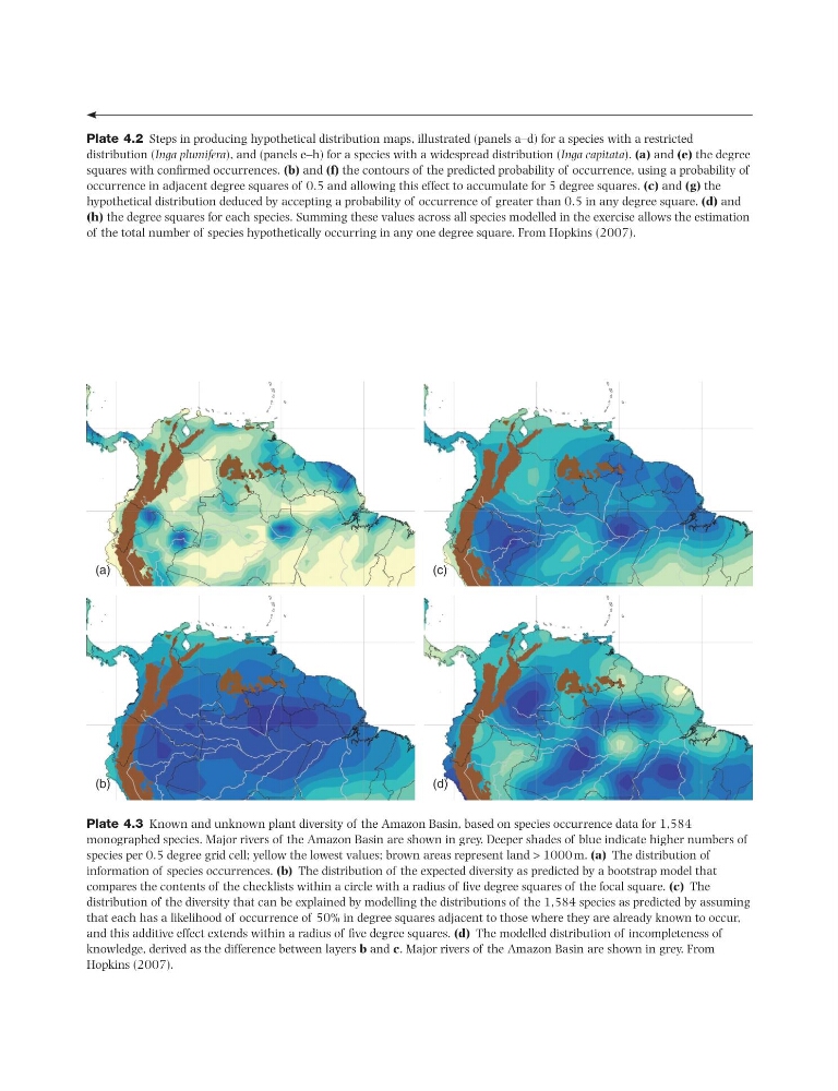
Plate 4.3 Known and unknown plant diversity of the Amazon Basin, based on species occurrence data for 1,584
monographed species. Major rivers of the Amazon Basin are shown in grey. Deeper shades of blue indicate higher numbers of
species per 0.5 degree grid cell; yellow the lowest values; brown areas represent land > 1000 m. (a) The distribution of
information of species occurrences. (b) The distribution of the expected diversity as predicted by a bootstrap model that
compares the contents of the checklists within a circle with a radius of fi ve degree squares of the focal square. (c) The
distribution of the diversity that can be explained by modelling the distributions of the 1,584 species as predicted by assuming
that each has a likelihood of occurrence of 50% in degree squares adjacent to those where they are already known to occur,
and this additive effect extends within a radius of fi ve degree squares. (d) The modelled distribution of incompleteness of
knowledge, derived as the difference between layers b and c. Major rivers of the Amazon Basin are shown in grey. From
Hopkins (2007).
distribution (Inga plumifera), and (panels e–h) for a species with a widespread distribution (Inga capitata). (a) and (e) the degree
squares with confi rmed occurrences. (b) and (f) the contours of the predicted probability of occurrence, using a probability of
occurrence in adjacent degree squares of 0.5 and allowing this effect to accumulate for 5 degree squares. (c) and (g) the
hypothetical distribution deduced by accepting a probability of occurrence of greater than 0.5 in any degree square. (d) and
(h) the degree squares for each species. Summing these values across all species modelled in the exercise allows the estimation
of the total number of species hypothetically occurring in any one degree square. From Hopkins (2007).
(a)
(b)
(c)
(d)
Plate 4.3 Known and unknown plant diversity of the Amazon Basin, based on species occurrence data for 1,584
monographed species. Major rivers of the Amazon Basin are shown in grey. Deeper shades of blue indicate higher numbers of
species per 0.5 degree grid cell; yellow the lowest values; brown areas represent land > 1000 m. (a) The distribution of
information of species occurrences. (b) The distribution of the expected diversity as predicted by a bootstrap model that
compares the contents of the checklists within a circle with a radius of fi ve degree squares of the focal square. (c) The
distribution of the diversity that can be explained by modelling the distributions of the 1,584 species as predicted by assuming
that each has a likelihood of occurrence of 50% in degree squares adjacent to those where they are already known to occur,
and this additive effect extends within a radius of fi ve degree squares. (d) The modelled distribution of incompleteness of
knowledge, derived as the difference between layers b and c. Major rivers of the Amazon Basin are shown in grey. From
Hopkins (2007).