

Murphy, Bro, and Stedmon
364
cross-validation used with a large data set, or even a small data set if it includes replicate
samples) (Westerhuis et al., 2008; Kjeldahla and Bro, 2010). This often leads to the selection of overfitted models that are likely to perform worse when making future predictions
than models that have fewer latent variables.
For the river and WTP sites, a five-component model has the lowest RMSECV; however, the two-component model appears to be a better choice, given that relatively small
gains in RMSECV (and the correlation coefficient, R
2 cv ) are obtained by including the last
three latent variables. For the estuary sites, a three- component model appears to be sufficient. Again, a seven-component model has lower RMSECV, yet only very small improvements in RMSECV are attained with the addition of many latent variables. A conservative
approach is thus to select two latent variables for the river and WTP model, and three for
the estuary model.
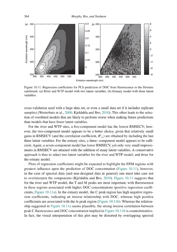
Plots of regression coefficients might be expected to highlight the EEM regions with
greatest influence upon the prediction of DOC concentration (Figure 10.11), however,
in the case of spectral data (and non-designed data in general) one must take care not
to overinterpret the components (Kjeldahla and Bro, 2010). Figure 10.11 suggests that
for the river and WTP model, the T and M peaks are most important, with fluorescence
in these regions associated with higher DOC concentrations (positive regression coefficients, Figure 10.11a). In the estuary model, the C peak region has high negative regression coefficients, indicating an inverse relationship with DOC, whereas high positive
coefficients are associated with the A-peak region (Figure 10.11b). Whereas the relationship suggested in Figure 10.11a seems plausible, the strong inverse correlation between
peak C fluorescence and DOC concentration implied in Figure 10.11b is counterintuitive.
In fact, the visual interpretation of this plot may be distorted by overlapping spectral
300 350 400 450 500 550
250
300
350
400
450
Excitation wavelength (nm)
Emission wavelength (nm)
300 350 400 450 500 550
250
300
350
400
450
0
0.05
0.1
0.15
0.2
0.25
0.3
−8
−6
−4
−2
0
2
4
6
8
(a)
(b)
Figure 10.11. Regression coefficients for PLS prediction of DOC from fluorescence in the Horsens
catchment. (a) River and WTP model with two latent variables. (b) Estuary model with three latent
variables.
364
cross-validation used with a large data set, or even a small data set if it includes replicate
samples) (Westerhuis et al., 2008; Kjeldahla and Bro, 2010). This often leads to the selection of overfitted models that are likely to perform worse when making future predictions
than models that have fewer latent variables.
For the river and WTP sites, a five-component model has the lowest RMSECV; however, the two-component model appears to be a better choice, given that relatively small
gains in RMSECV (and the correlation coefficient, R
2 cv ) are obtained by including the last
three latent variables. For the estuary sites, a three- component model appears to be sufficient. Again, a seven-component model has lower RMSECV, yet only very small improvements in RMSECV are attained with the addition of many latent variables. A conservative
approach is thus to select two latent variables for the river and WTP model, and three for
the estuary model.
Plots of regression coefficients might be expected to highlight the EEM regions with
greatest influence upon the prediction of DOC concentration (Figure 10.11), however,
in the case of spectral data (and non-designed data in general) one must take care not
to overinterpret the components (Kjeldahla and Bro, 2010). Figure 10.11 suggests that
for the river and WTP model, the T and M peaks are most important, with fluorescence
in these regions associated with higher DOC concentrations (positive regression coefficients, Figure 10.11a). In the estuary model, the C peak region has high negative regression coefficients, indicating an inverse relationship with DOC, whereas high positive
coefficients are associated with the A-peak region (Figure 10.11b). Whereas the relationship suggested in Figure 10.11a seems plausible, the strong inverse correlation between
peak C fluorescence and DOC concentration implied in Figure 10.11b is counterintuitive.
In fact, the visual interpretation of this plot may be distorted by overlapping spectral
300 350 400 450 500 550
250
300
350
400
450
Excitation wavelength (nm)
Emission wavelength (nm)
300 350 400 450 500 550
250
300
350
400
450
0
0.05
0.1
0.15
0.2
0.25
0.3
−8
−6
−4
−2
0
2
4
6
8
(a)
(b)
Figure 10.11. Regression coefficients for PLS prediction of DOC from fluorescence in the Horsens
catchment. (a) River and WTP model with two latent variables. (b) Estuary model with three latent
variables.