

This can be solved by using the product rule:
(12.22)
letting
u = x
2
du = 2x dx d9 = e
−2x dx 9 = −e
−2x
/2
(12.23)
and another substitution
u = x du = dx d9 = e
−2x dx 9 = −e
−2x
/2
(12.24)
(12.25)
(12.26)
So there is only a 32% probability of finding the electron with the radius a 0 .
Perhaps more useful is the average (or expectation) value of the radius.
We can calculate it as:
(12.27)
Let x = r/a 0 and then use the same approach as above:
(12.28)
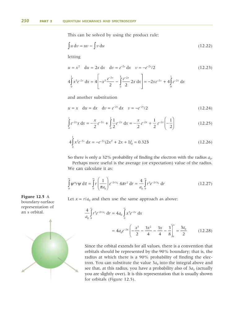
Since the orbital extends for all values, there is a convention that
orbitals should be represented by the 90% boundary; that is, the
radius at which there is a 90% probability of finding the electron. You can substitute the value 3a 0 into the integral above and
see that, at this radius, you have a probability also of 3a 0 (actually
you are slightly over). It is this representation that is usually shown
for orbitals (Figure 12.5).
4 0
2
a e
−
=
x x
x
x
x
a
−
−
−
−
⎛
⎝
⎜ ⎜
⎞
⎠
⎟ ⎟ =
∞
3
2
0
0
2
3
4
3
4
3
8
3
2
4
4
0
3
0
2
0
3 2
0
0
a
r e
r
a x e
x
r a
x
∞
−
−
∞
∫
∫
=
/ d
d
ψ ψ τ
π
π
* d
d
r
r
a
e
r r
r a
/
=
⎛
⎝
⎜ ⎜
⎞
⎠
⎟ ⎟
=
−
∞
∞
∫
∫
1
4
0
2
0
0
2
0
/
4
0
3
0
2 0
a
r e
r
r a
∞
−
∫
d
4
2
2
1
0 3 2
2 2
0
1
2
2
0
1
x e
x
e
x
x
x
x
−
−
∫
= −
+
+
=
d
(
)
. 3 3
e x x
x e
e
x
x e
x
x
x
−
−
−
−
= −
+
= −
∫
∫
2
0
1
2
2
0
1
2
2
1
2
2
d
d
x x
x
e
+
−
⎛
⎝
⎜ ⎜
⎞
⎠
⎟ ⎟
−
1
2
1
2
2
4
4
2
2
2
2
0
1
2
2
2
2
0
1
x e
x
x
e
e
x x
x
x
x
∫
∫
−
−
−
= −
−
⎡
⎣
⎢
⎢
d
d
⎤ ⎤
⎦
⎥
⎥
= −
+
−
−
∫
2
4
2
2
0
1
xe
e
x
x
x d
u
u
u
d
d
9
9
9
=
− ∫
∫
250
PART 2
QUANTUM MECHANICS AND SPECTROSCOPY
Figure 12.5 A
boundary-surface
representation of
an s orbital.
9781405124362_4_012.qxd 4/29/08 9:11 Page 250
(12.22)
letting
u = x
2
du = 2x dx d9 = e
−2x dx 9 = −e
−2x
/2
(12.23)
and another substitution
u = x du = dx d9 = e
−2x dx 9 = −e
−2x
/2
(12.24)
(12.25)
(12.26)
So there is only a 32% probability of finding the electron with the radius a 0 .
Perhaps more useful is the average (or expectation) value of the radius.
We can calculate it as:
(12.27)
Let x = r/a 0 and then use the same approach as above:
(12.28)
Since the orbital extends for all values, there is a convention that
orbitals should be represented by the 90% boundary; that is, the
radius at which there is a 90% probability of finding the electron. You can substitute the value 3a 0 into the integral above and
see that, at this radius, you have a probability also of 3a 0 (actually
you are slightly over). It is this representation that is usually shown
for orbitals (Figure 12.5).
4 0
2
a e
−
=
x x
x
x
x
a
−
−
−
−
⎛
⎝
⎜ ⎜
⎞
⎠
⎟ ⎟ =
∞
3
2
0
0
2
3
4
3
4
3
8
3
2
4
4
0
3
0
2
0
3 2
0
0
a
r e
r
a x e
x
r a
x
∞
−
−
∞
∫
∫
=
/ d
d
ψ ψ τ
π
π
* d
d
r
r
a
e
r r
r a
/
=
⎛
⎝
⎜ ⎜
⎞
⎠
⎟ ⎟
=
−
∞
∞
∫
∫
1
4
0
2
0
0
2
0
/
4
0
3
0
2 0
a
r e
r
r a
∞
−
∫
d
4
2
2
1
0 3 2
2 2
0
1
2
2
0
1
x e
x
e
x
x
x
x
−
−
∫
= −
+
+
=
d
(
)
. 3 3
e x x
x e
e
x
x e
x
x
x
−
−
−
−
= −
+
= −
∫
∫
2
0
1
2
2
0
1
2
2
1
2
2
d
d
x x
x
e
+
−
⎛
⎝
⎜ ⎜
⎞
⎠
⎟ ⎟
−
1
2
1
2
2
4
4
2
2
2
2
0
1
2
2
2
2
0
1
x e
x
x
e
e
x x
x
x
x
∫
∫
−
−
−
= −
−
⎡
⎣
⎢
⎢
d
d
⎤ ⎤
⎦
⎥
⎥
= −
+
−
−
∫
2
4
2
2
0
1
xe
e
x
x
x d
u
u
u
d
d
9
9
9
=
− ∫
∫
250
PART 2
QUANTUM MECHANICS AND SPECTROSCOPY
Figure 12.5 A
boundary-surface
representation of
an s orbital.
9781405124362_4_012.qxd 4/29/08 9:11 Page 250