

Relative error of bottom albedo (%)
Relative error of z B
(%)
100
75
50
25
0
-25
-50
-50
-25
0
2 5
50
75
100
5 m
z B =1 m
A
ERR_FA2 | 25.9.2003
Bottom depth z B (m)
Relative error of z B
(%)
0
5
1 0
1 5
2 0
-100
-50
0
50
100
FIG9B | 24.5.2005
B
chara
pect
perf
const
sand
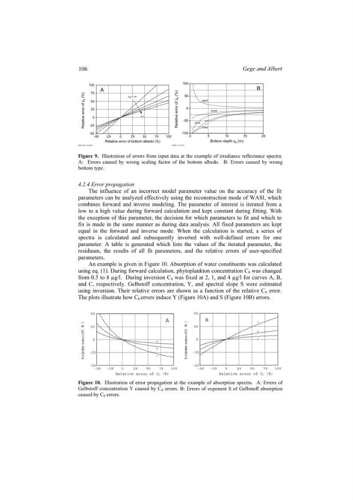
Figure 9. Illustration of errors from input data at the example of irradiance reflectance spectra.
A: Errors caused by wrong scaling factor of the bottom albedo. B: Errors caused by wrong
bottom type.
4.2.4 Error propagation
The influence of an incorrect model parameter value on the accuracy of the fit
parameters can be analyzed effectively using the reconstruction mode of WASI, which
combines forward and inverse modeling. The parameter of interest is iterated from a
low to a high value during forward calculation and kept constant during fitting. With
the exception of this parameter, the decision for which parameters to fit and which to
fix is made in the same manner as during data analysis. All fixed parameters are kept
equal in the forward and inverse mode. When the calculation is started, a series of
spectra is calculated and subsequently inverted with well-defined errors for one
parameter. A table is generated which lists the values of the iterated parameter, the
residuum, the results of all fit parameters, and the relative errors of user-specified
parameters.
An example is given in Figure 10. Absorption of water constituents was calculated
using eq. (1). During forward calculation, phytoplankton concentration C 0 was changed
from 0.5 to 8 µg/l. During inversion C 0 was fixed at 2, 1, and 4 µg/l for curves A, B,
and C, respectively. Gelbstoff concentration, Y, and spectral slope S were estimated
using inversion. Their relative errors are shown as a function of the relative C 0 error.
The plots illustrate how C 0 errors induce Y (Figure 10A) and S (Figure 10B) errors.
50
25
0
-25
-50
-50
-25
0
25
50
75
100
A
C
B
Relative error of C0 (%)
R el at
i ve errorofY (%
)
A
50
25
0
-25
-50
-50
-25
0
25
50
75
100
A
C
B
B
Relative error of C0 (%)
R el at
i ve errorofS (%
)
Figure 10. Illustration of error propagation at the example of absorption spectra. A: Errors of
Gelbstoff concentration Y caused by C 0 errors. B: Errors of exponent S of Gelbstoff absorption
caused by C 0 errors.
106
Gege and Albert
Relative error of z B
(%)
100
75
50
25
0
-25
-50
-50
-25
0
2 5
50
75
100
5 m
z B =1 m
A
ERR_FA2 | 25.9.2003
Bottom depth z B (m)
Relative error of z B
(%)
0
5
1 0
1 5
2 0
-100
-50
0
50
100
FIG9B | 24.5.2005
B
chara
pect
perf
const
sand
Figure 9. Illustration of errors from input data at the example of irradiance reflectance spectra.
A: Errors caused by wrong scaling factor of the bottom albedo. B: Errors caused by wrong
bottom type.
4.2.4 Error propagation
The influence of an incorrect model parameter value on the accuracy of the fit
parameters can be analyzed effectively using the reconstruction mode of WASI, which
combines forward and inverse modeling. The parameter of interest is iterated from a
low to a high value during forward calculation and kept constant during fitting. With
the exception of this parameter, the decision for which parameters to fit and which to
fix is made in the same manner as during data analysis. All fixed parameters are kept
equal in the forward and inverse mode. When the calculation is started, a series of
spectra is calculated and subsequently inverted with well-defined errors for one
parameter. A table is generated which lists the values of the iterated parameter, the
residuum, the results of all fit parameters, and the relative errors of user-specified
parameters.
An example is given in Figure 10. Absorption of water constituents was calculated
using eq. (1). During forward calculation, phytoplankton concentration C 0 was changed
from 0.5 to 8 µg/l. During inversion C 0 was fixed at 2, 1, and 4 µg/l for curves A, B,
and C, respectively. Gelbstoff concentration, Y, and spectral slope S were estimated
using inversion. Their relative errors are shown as a function of the relative C 0 error.
The plots illustrate how C 0 errors induce Y (Figure 10A) and S (Figure 10B) errors.
50
25
0
-25
-50
-50
-25
0
25
50
75
100
A
C
B
Relative error of C0 (%)
R el at
i ve errorofY (%
)
A
50
25
0
-25
-50
-50
-25
0
25
50
75
100
A
C
B
B
Relative error of C0 (%)
R el at
i ve errorofS (%
)
Figure 10. Illustration of error propagation at the example of absorption spectra. A: Errors of
Gelbstoff concentration Y caused by C 0 errors. B: Errors of exponent S of Gelbstoff absorption
caused by C 0 errors.
106
Gege and Albert