

= 2 nm, noise = 0.002 m -1
100
60
20
-20
-60
-100
0.1
1
10
100
100
60
20
-20
-60
-100
0.1
1
10
100
100
60
20
-20
-60
-100
0.1
1
10
100
100
60
20
-20
-60
-100
0.1
1
10
100
Concentration C 0 (ug/l)
Concentration C 0 (ug/l)
Concentration C 0 (ug/l)
Concentration C 0 (ug/l)
= 2 nm, noise = 0.02 m -1
= 20 nm, noise = 0.002 m -1
= 20 nm, noise = 0.02 m -1
Relative error of C
0 (%)
Relative error of C
0 (%)
Relative error of C
0 (%)
Relative error of C
0 (%)
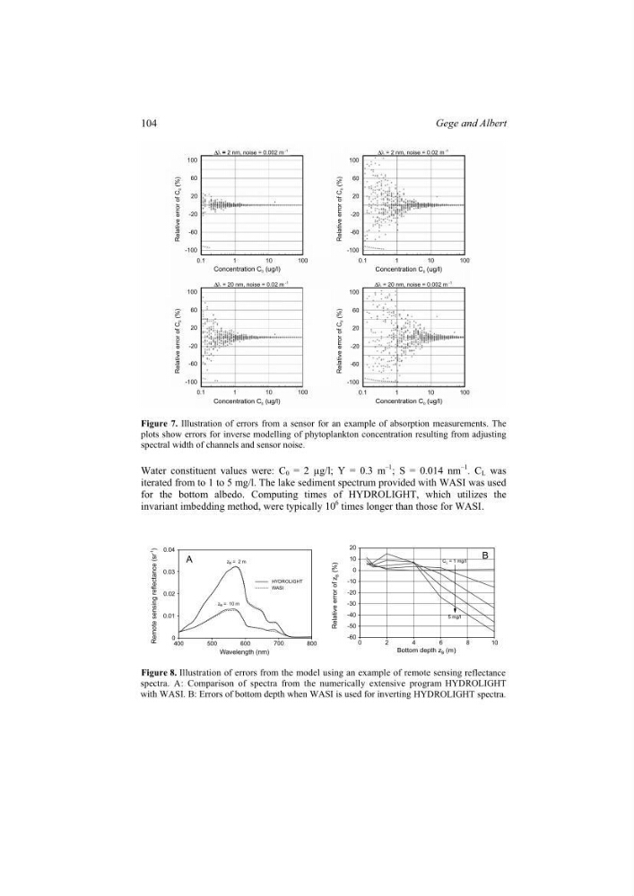
Figure 7. Illustration of errors from a sensor for an example of absorption measurements. The
plots show errors for inverse modelling of phytoplankton concentration resulting from adjusting
spectral width of channels and sensor noise.
Water constituent values were: C 0 = 2 µg/l; Y = 0.3 m
–1 ; S = 0.014 nm
–1
. C L was
iterated from to 1 to 5 mg/l. The lake sediment spectrum provided with WASI was used
for the bottom albedo. Computing times of HYDROLIGHT, which utilizes the
invariant imbedding method, were typically 10
6 times longer than those for WASI.
Wavelength (nm)
Remote sensing reflectance (sr
-1
)
0.04
0.03
0.02
0.01
0
400
500
600
700
800
z B = 2 m
z B = 10 m
HYDROLIGHT
WASI
A
20
10
0
-10
-20
-30
-40
-50
-60
0
2
4
6
8
10
5 mg/l
C L = 1 mg/l
B
Bottom depth z B (m)
Relative error of z
B (%)
reflectance
HYDROLIGHT
HYDROLIGHT spectra.
Figure 8. Illustration of errors from the model using an example of remote sensing
spectra. A: Comparison of spectra from the numerically extensive program
with WASI. B: Errors of bottom depth when WASI is used for inverting
104
Gege and Albert
100
60
20
-20
-60
-100
0.1
1
10
100
100
60
20
-20
-60
-100
0.1
1
10
100
100
60
20
-20
-60
-100
0.1
1
10
100
100
60
20
-20
-60
-100
0.1
1
10
100
Concentration C 0 (ug/l)
Concentration C 0 (ug/l)
Concentration C 0 (ug/l)
Concentration C 0 (ug/l)
= 2 nm, noise = 0.02 m -1
= 20 nm, noise = 0.002 m -1
= 20 nm, noise = 0.02 m -1
Relative error of C
0 (%)
Relative error of C
0 (%)
Relative error of C
0 (%)
Relative error of C
0 (%)
Figure 7. Illustration of errors from a sensor for an example of absorption measurements. The
plots show errors for inverse modelling of phytoplankton concentration resulting from adjusting
spectral width of channels and sensor noise.
Water constituent values were: C 0 = 2 µg/l; Y = 0.3 m
–1 ; S = 0.014 nm
–1
. C L was
iterated from to 1 to 5 mg/l. The lake sediment spectrum provided with WASI was used
for the bottom albedo. Computing times of HYDROLIGHT, which utilizes the
invariant imbedding method, were typically 10
6 times longer than those for WASI.
Wavelength (nm)
Remote sensing reflectance (sr
-1
)
0.04
0.03
0.02
0.01
0
400
500
600
700
800
z B = 2 m
z B = 10 m
HYDROLIGHT
WASI
A
20
10
0
-10
-20
-30
-40
-50
-60
0
2
4
6
8
10
5 mg/l
C L = 1 mg/l
B
Bottom depth z B (m)
Relative error of z
B (%)
reflectance
HYDROLIGHT
HYDROLIGHT spectra.
Figure 8. Illustration of errors from the model using an example of remote sensing
spectra. A: Comparison of spectra from the numerically extensive program
with WASI. B: Errors of bottom depth when WASI is used for inverting
104
Gege and Albert