

Exponent S (nm -1 )
Concentration Y (m
-1
)
0,010
0,012
0,014
0,016
0,018
0,020
0,0
0,1
0,2
0,3
0,4
0,5
0,6
0,0020
0,0015
5E-4
0,0015
0,0020
1E-3
Exponent S (nm -1 )
Concentration Y (m
-1
)
0,010
0,012
0,014
0,016
0,018
0,020
0,0
0,1
0,2
0,3
0,4
0,5
0,6
0,020
0,020
0,015
0,0050
0,010
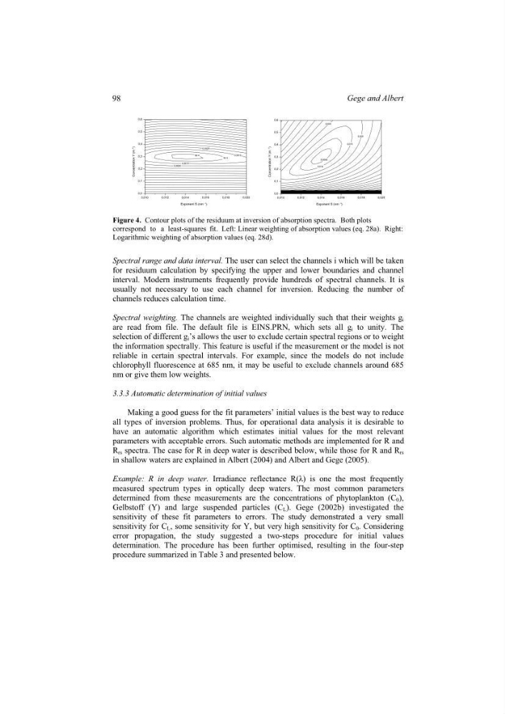
Figure 4. Contour plots of the residuum at inversion of absorption spectra. Both plots
correspond to a least-squares fit. Left: Linear weighting of absorption values (eq. 28a). Right:
Logarithmic weighting of absorption values (eq. 28d).
Spectral range and data interval. The user can select the channels i which will be taken
for residuum calculation by specifying the upper and lower boundaries and channel
interval. Modern instruments frequently provide hundreds of spectral channels. It is
usually not necessary to use each channel for inversion. Reducing the number of
channels reduces calculation time.
Spectral weighting. The channels are weighted individually such that their weights g i
are read from file. The default file is EINS.PRN, which sets all g i to unity. The
selection of different g i ’s allows the user to exclude certain spectral regions or to weight
the information spectrally. This feature is useful if the measurement or the model is not
reliable in certain spectral intervals. For example, since the models do not include
chlorophyll fluorescence at 685 nm, it may be useful to exclude channels around 685
nm or give them low weights.
3.3.3 Automatic determination of initial values
Making a good guess for the fit parameters’ initial values is the best way to reduce
all types of inversion problems. Thus, for operational data analysis it is desirable to
have an automatic algorithm which estimates initial values for the most relevant
parameters with acceptable errors. Such automatic methods are implemented for R and
R rs spectra. The case for R in deep water is described below, while those for R and R rs
in shallow waters are explained in Albert (2004) and Albert and Gege (2005).
Example: R in deep water. Irradiance reflectance R(Ȝ) is one the most frequently
measured spectrum types in optically deep waters. The most common parameters
determined from these measurements are the concentrations of phytoplankton (C 0 ),
Gelbstoff (Y) and large suspended particles (C L ). Gege (2002b) investigated the
sensitivity of these fit parameters to errors. The study demonstrated a very small
sensitivity for C L , some sensitivity for Y, but very high sensitivity for C 0 . Considering
error propagation, the study suggested a two-steps procedure for initial values
determination. The procedure has been further optimised, resulting in the four-step
procedure summarized in Table 3 and presented below.
98
Gege and Albert
Concentration Y (m
-1
)
0,010
0,012
0,014
0,016
0,018
0,020
0,0
0,1
0,2
0,3
0,4
0,5
0,6
0,0020
0,0015
5E-4
0,0015
0,0020
1E-3
Exponent S (nm -1 )
Concentration Y (m
-1
)
0,010
0,012
0,014
0,016
0,018
0,020
0,0
0,1
0,2
0,3
0,4
0,5
0,6
0,020
0,020
0,015
0,0050
0,010
Figure 4. Contour plots of the residuum at inversion of absorption spectra. Both plots
correspond to a least-squares fit. Left: Linear weighting of absorption values (eq. 28a). Right:
Logarithmic weighting of absorption values (eq. 28d).
Spectral range and data interval. The user can select the channels i which will be taken
for residuum calculation by specifying the upper and lower boundaries and channel
interval. Modern instruments frequently provide hundreds of spectral channels. It is
usually not necessary to use each channel for inversion. Reducing the number of
channels reduces calculation time.
Spectral weighting. The channels are weighted individually such that their weights g i
are read from file. The default file is EINS.PRN, which sets all g i to unity. The
selection of different g i ’s allows the user to exclude certain spectral regions or to weight
the information spectrally. This feature is useful if the measurement or the model is not
reliable in certain spectral intervals. For example, since the models do not include
chlorophyll fluorescence at 685 nm, it may be useful to exclude channels around 685
nm or give them low weights.
3.3.3 Automatic determination of initial values
Making a good guess for the fit parameters’ initial values is the best way to reduce
all types of inversion problems. Thus, for operational data analysis it is desirable to
have an automatic algorithm which estimates initial values for the most relevant
parameters with acceptable errors. Such automatic methods are implemented for R and
R rs spectra. The case for R in deep water is described below, while those for R and R rs
in shallow waters are explained in Albert (2004) and Albert and Gege (2005).
Example: R in deep water. Irradiance reflectance R(Ȝ) is one the most frequently
measured spectrum types in optically deep waters. The most common parameters
determined from these measurements are the concentrations of phytoplankton (C 0 ),
Gelbstoff (Y) and large suspended particles (C L ). Gege (2002b) investigated the
sensitivity of these fit parameters to errors. The study demonstrated a very small
sensitivity for C L , some sensitivity for Y, but very high sensitivity for C 0 . Considering
error propagation, the study suggested a two-steps procedure for initial values
determination. The procedure has been further optimised, resulting in the four-step
procedure summarized in Table 3 and presented below.
98
Gege and Albert