

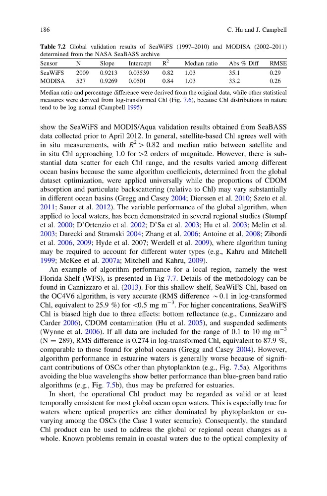
show the SeaWiFS and MODIS/Aqua validation results obtained from SeaBASS
data collected prior to April 2012. In general, satellite-based Chl agrees well with
in situ measurements, with R
2 [ 0.82 and median ratio between satellite and
in situ Chl approaching 1.0 for [2 orders of magnitude. However, there is substantial data scatter for each Chl range, and the results varied among different
ocean basins because the same algorithm coefficients, determined from the global
dataset optimization, were applied universally while the proportions of CDOM
absorption and particulate backscattering (relative to Chl) may vary substantially
in different ocean basins (Gregg and Casey 2004; Dierssen et al. 2010; Szeto et al.
2011; Sauer et al. 2012). The variable performance of the global algorithm, when
applied to local waters, has been demonstrated in several regional studies (Stumpf
et al. 2000; D’Ortenzio et al. 2002; D’Sa et al. 2003; Hu et al. 2003; Melin et al.
2003; Darecki and Stramski 2004; Zhang et al. 2006; Antoine et al. 2008; Zibordi
et al. 2006, 2009; Hyde et al. 2007; Werdell et al. 2009), where algorithm tuning
may be required to account for different water types (e.g., Kahru and Mitchell
1999; McKee et al. 2007a; Mitchell and Kahru, 2009).
An example of algorithm performance for a local region, namely the west
Florida Shelf (WFS), is presented in Fig 7.7. Details of the methodology can be
found in Cannizzaro et al. (2013). For this shallow shelf, SeaWiFS Chl, based on
the OC4V6 algorithm, is very accurate (RMS difference *0.1 in log-transformed
Chl, equivalent to 25.9 %) for \0.5 mg m
-3 . For higher concentrations, SeaWiFS
Chl is biased high due to three effects: bottom reflectance (e.g., Cannizzaro and
Carder 2006), CDOM contamination (Hu et al. 2005), and suspended sediments
(Wynne et al. 2006). If all data are included for the range of 0.1 to 10 mg m
-3
(N = 289), RMS difference is 0.274 in log-transformed Chl, equivalent to 87.9 %,
comparable to those found for global oceans (Gregg and Casey 2004). However,
algorithm performance in estuarine waters is generally worse because of significant contributions of OSCs other than phytoplankton (e.g., Fig. 7.5a). Algorithms
avoiding the blue wavelengths show better performance than blue-green band ratio
algorithms (e.g., Fig. 7.5b), thus may be preferred for estuaries.
In short, the operational Chl product may be regarded as valid or at least
temporally consistent for most global ocean open waters. This is especially true for
waters where optical properties are either dominated by phytoplankton or covarying among the OSCs (the Case I water scenario). Consequently, the standard
Chl product can be used to address the global or regional ocean changes as a
whole. Known problems remain in coastal waters due to the optical complexity of
Table 7.2 Global validation results of SeaWiFS (1997–2010) and MODISA (2002–2011)
determined from the NASA SeaBASS archive
Sensor
N
Slope
Intercept
R
2
Median ratio
Abs % Diff
RMSE
SeaWiFS
2009
0.9213
0.03539
0.82
1.03
35.1
0.29
MODISA
527
0.9269
0.0501
0.84
1.03
33.2
0.26
Median ratio and percentage difference were derived from the original data, while other statistical
measures were derived from log-transformed Chl (Fig. 7.6), because Chl distributions in nature
tend to be log normal (Campbell 1995)
186
C. Hu and J. Campbell
data collected prior to April 2012. In general, satellite-based Chl agrees well with
in situ measurements, with R
2 [ 0.82 and median ratio between satellite and
in situ Chl approaching 1.0 for [2 orders of magnitude. However, there is substantial data scatter for each Chl range, and the results varied among different
ocean basins because the same algorithm coefficients, determined from the global
dataset optimization, were applied universally while the proportions of CDOM
absorption and particulate backscattering (relative to Chl) may vary substantially
in different ocean basins (Gregg and Casey 2004; Dierssen et al. 2010; Szeto et al.
2011; Sauer et al. 2012). The variable performance of the global algorithm, when
applied to local waters, has been demonstrated in several regional studies (Stumpf
et al. 2000; D’Ortenzio et al. 2002; D’Sa et al. 2003; Hu et al. 2003; Melin et al.
2003; Darecki and Stramski 2004; Zhang et al. 2006; Antoine et al. 2008; Zibordi
et al. 2006, 2009; Hyde et al. 2007; Werdell et al. 2009), where algorithm tuning
may be required to account for different water types (e.g., Kahru and Mitchell
1999; McKee et al. 2007a; Mitchell and Kahru, 2009).
An example of algorithm performance for a local region, namely the west
Florida Shelf (WFS), is presented in Fig 7.7. Details of the methodology can be
found in Cannizzaro et al. (2013). For this shallow shelf, SeaWiFS Chl, based on
the OC4V6 algorithm, is very accurate (RMS difference *0.1 in log-transformed
Chl, equivalent to 25.9 %) for \0.5 mg m
-3 . For higher concentrations, SeaWiFS
Chl is biased high due to three effects: bottom reflectance (e.g., Cannizzaro and
Carder 2006), CDOM contamination (Hu et al. 2005), and suspended sediments
(Wynne et al. 2006). If all data are included for the range of 0.1 to 10 mg m
-3
(N = 289), RMS difference is 0.274 in log-transformed Chl, equivalent to 87.9 %,
comparable to those found for global oceans (Gregg and Casey 2004). However,
algorithm performance in estuarine waters is generally worse because of significant contributions of OSCs other than phytoplankton (e.g., Fig. 7.5a). Algorithms
avoiding the blue wavelengths show better performance than blue-green band ratio
algorithms (e.g., Fig. 7.5b), thus may be preferred for estuaries.
In short, the operational Chl product may be regarded as valid or at least
temporally consistent for most global ocean open waters. This is especially true for
waters where optical properties are either dominated by phytoplankton or covarying among the OSCs (the Case I water scenario). Consequently, the standard
Chl product can be used to address the global or regional ocean changes as a
whole. Known problems remain in coastal waters due to the optical complexity of
Table 7.2 Global validation results of SeaWiFS (1997–2010) and MODISA (2002–2011)
determined from the NASA SeaBASS archive
Sensor
N
Slope
Intercept
R
2
Median ratio
Abs % Diff
RMSE
SeaWiFS
2009
0.9213
0.03539
0.82
1.03
35.1
0.29
MODISA
527
0.9269
0.0501
0.84
1.03
33.2
0.26
Median ratio and percentage difference were derived from the original data, while other statistical
measures were derived from log-transformed Chl (Fig. 7.6), because Chl distributions in nature
tend to be log normal (Campbell 1995)
186
C. Hu and J. Campbell