

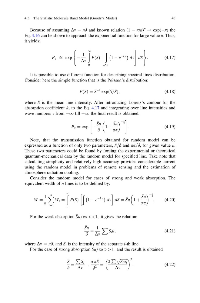
Because of assuming Dn ¼ nd and known relation (1 À x/n)
n ! exp(Àx) the
Eq. 4.16 can be shown to approach the exponential function for large value n. Thus,
it yields:
P n ffi exp À
1
Dn
ð
1
0
PðSÞ
ð
Dn
1 À e
Àku
À
Á
dn
2
4
3
5 dS
8
<
:
9
=
;
:
(4.17)
It is possible to use different function for describing spectral lines distribution.
Consider here the simple function that is the Poisson’s distribution:
PðSÞ ¼
S
À1 expðS
S
= Þ;
(4.18)
where
S is the mean line intensity. After introducing Lorenz’s contour for the
absorption coefficient k n to the Eq. 4.17 and integrating over line intensities and
wave numbers n from À1 till þ1 the final result is obtained.
P n ¼ exp À
Su
d
1 þ
Su
pa
À
1
2
"
#
:
(4.19)
Note, that the transmission function obtained for random model can be
expressed as a function of only two parameters,
S d
= and pa d
= , for given value u.
These two parameters could be found by forcing the experimental or theoretical
quantum-mechanical data by the random model for specified line. Take note that
calculating simplicity and relatively high accuracy provides considerable current
using the random model in problems of remote sensing and the estimation of
atmosphere radiation cooling.
Consider the random model for cases of strong and weak absorption. The
equivalent width of n lines is to be defined by:
W ¼
1
n
X n
i¼1
W i ¼
ð
1
0
PðSÞ
ð
1 À e
Àk u
À
Á
dn
!
dS ¼
Su 1 þ
Su
pa
À
1
2
;
(4.20)
For the weak absorption Su pa
= <<1; it gives the relation:
Su
d
¼
1
Dn
X
S i u;
(4.21)
where Dn ¼ nd, and S i is the intensity of the separate i-th line.
For the case of strong absorption Su pa
= >>1; and the result is obtained
S
d
¼
P
S i
Dn
;
a p
S
d
2
¼
2
P ffiffiffiffiffiffiffi ffi
S i a i
p
Dn
2
:
(4.22)
4.3 The Statistic Molecule Band Model (Goody’s Model)
43
n ! exp(Àx) the
Eq. 4.16 can be shown to approach the exponential function for large value n. Thus,
it yields:
P n ffi exp À
1
Dn
ð
1
0
PðSÞ
ð
Dn
1 À e
Àku
À
Á
dn
2
4
3
5 dS
8
<
:
9
=
;
:
(4.17)
It is possible to use different function for describing spectral lines distribution.
Consider here the simple function that is the Poisson’s distribution:
PðSÞ ¼
S
À1 expðS
S
= Þ;
(4.18)
where
S is the mean line intensity. After introducing Lorenz’s contour for the
absorption coefficient k n to the Eq. 4.17 and integrating over line intensities and
wave numbers n from À1 till þ1 the final result is obtained.
P n ¼ exp À
Su
d
1 þ
Su
pa
À
1
2
"
#
:
(4.19)
Note, that the transmission function obtained for random model can be
expressed as a function of only two parameters,
S d
= and pa d
= , for given value u.
These two parameters could be found by forcing the experimental or theoretical
quantum-mechanical data by the random model for specified line. Take note that
calculating simplicity and relatively high accuracy provides considerable current
using the random model in problems of remote sensing and the estimation of
atmosphere radiation cooling.
Consider the random model for cases of strong and weak absorption. The
equivalent width of n lines is to be defined by:
W ¼
1
n
X n
i¼1
W i ¼
ð
1
0
PðSÞ
ð
1 À e
Àk u
À
Á
dn
!
dS ¼
Su 1 þ
Su
pa
À
1
2
;
(4.20)
For the weak absorption Su pa
= <<1; it gives the relation:
Su
d
¼
1
Dn
X
S i u;
(4.21)
where Dn ¼ nd, and S i is the intensity of the separate i-th line.
For the case of strong absorption Su pa
= >>1; and the result is obtained
S
d
¼
P
S i
Dn
;
a p
S
d
2
¼
2
P ffiffiffiffiffiffiffi ffi
S i a i
p
Dn
2
:
(4.22)
4.3 The Statistic Molecule Band Model (Goody’s Model)
43