

When conducting remote sensing, it is mandatory to also consider the optical properties of the wind-roughened water surface as these characteristics/
parameters determine the proportion of the desired signal in the total radiant
signal captured by the remote sensor. However, within the framework of these
teaching labs, for simplicity reasons we’ll confine ourselves to the case of calm
water surface.
The standard bio-optical water quality retrieval algorithms developed so far
prove to be untenable unless they are employed strictly to off-coastal/ open ocean
waters (so called case I waters). This is due to hydro-optically complexity of
composition of inland and marine coastal waters (so called case 2 waters), which
is further accentuated by the multitude of mechanisms of light interactions with the
aquatic medium and pathways of formation of the water leaving radiant signal.
Collectively, these factors render simplistic/case I water algorithms inadequate as
they are traditionally based on band-ratio parameterizations operating with light
signals in the blue and green spectral regions.
That is why when sounding case 2 waters, more accurate retrieval results can
be attained employing more sophisticated mathematical approaches, among which
is the Levenberg-Marquardt method of multivariate optimization. This procedure
is based on minimization of squared sums of residuals between the measured
and simulated/theoretical water volume diffuse reflectance. Practice No.10 is dedicated to this method and its application
Because all three Practice 15–17 are thematically closely interrelated, it is
recommended to study the basic theoretical part of Chap. 16 before preparing to
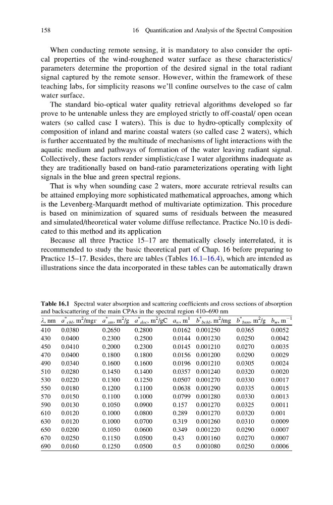
Practice 15–17. Besides, there are tables (Tables 16.1–16.4), which are intended as
illustrations since the data incorporated in these tables can be automatically drawn
Table 16.1 Spectral water absorption and scattering coefficients and cross sections of absorption
and backscattering of the main CPAs in the spectral region 410–690 nm
l, nm a
*
chl , m
2 /mgг a
*
sm , m
2 /g a
*
doc , m
2 /gC a w , m
1 b
*
bchl , m
2 /mg b
*
bsm , m
2 /g b w , m
À1
410
0.0380
0.2650
0.2800
0.0162 0.001250
0.0365
0.0052
430
0.0400
0.2300
0.2500
0.0144 0.001230
0.0250
0.0042
450
0.0410
0.2000
0.2300
0.0145 0.001210
0.0270
0.0035
470
0.0400
0.1800
0.1800
0.0156 0.001200
0.0290
0.0029
490
0.0340
0.1600
0.1600
0.0196 0.001210
0.0305
0.0024
510
0.0280
0.1450
0.1400
0.0357 0.001240
0.0320
0.0020
530
0.0220
0.1300
0.1250
0.0507 0.001270
0.0330
0.0017
550
0.0180
0.1200
0.1100
0.0638 0.001290
0.0335
0.0015
570
0.0150
0.1100
0.1000
0.0799 0.001280
0.0330
0.0013
590
0.0130
0.1050
0.0900
0.157 0.001270
0.0325
0.0011
610
0.0120
0.1000
0.0800
0.289 0.001270
0.0320
0.001
630
0.0120
0.1000
0.0700
0.319 0.001260
0.0310
0.0009
650
0.0200
0.1050
0.0600
0.349 0.001220
0.0290
0.0007
670
0.0250
0.1150
0.0500
0.43
0.001160
0.0270
0.0007
690
0.0160
0.1250
0.0500
0.5
0.001080
0.0250
0.0006
158
16 Quantification and Analysis of the Spectral Composition
parameters determine the proportion of the desired signal in the total radiant
signal captured by the remote sensor. However, within the framework of these
teaching labs, for simplicity reasons we’ll confine ourselves to the case of calm
water surface.
The standard bio-optical water quality retrieval algorithms developed so far
prove to be untenable unless they are employed strictly to off-coastal/ open ocean
waters (so called case I waters). This is due to hydro-optically complexity of
composition of inland and marine coastal waters (so called case 2 waters), which
is further accentuated by the multitude of mechanisms of light interactions with the
aquatic medium and pathways of formation of the water leaving radiant signal.
Collectively, these factors render simplistic/case I water algorithms inadequate as
they are traditionally based on band-ratio parameterizations operating with light
signals in the blue and green spectral regions.
That is why when sounding case 2 waters, more accurate retrieval results can
be attained employing more sophisticated mathematical approaches, among which
is the Levenberg-Marquardt method of multivariate optimization. This procedure
is based on minimization of squared sums of residuals between the measured
and simulated/theoretical water volume diffuse reflectance. Practice No.10 is dedicated to this method and its application
Because all three Practice 15–17 are thematically closely interrelated, it is
recommended to study the basic theoretical part of Chap. 16 before preparing to
Practice 15–17. Besides, there are tables (Tables 16.1–16.4), which are intended as
illustrations since the data incorporated in these tables can be automatically drawn
Table 16.1 Spectral water absorption and scattering coefficients and cross sections of absorption
and backscattering of the main CPAs in the spectral region 410–690 nm
l, nm a
*
chl , m
2 /mgг a
*
sm , m
2 /g a
*
doc , m
2 /gC a w , m
1 b
*
bchl , m
2 /mg b
*
bsm , m
2 /g b w , m
À1
410
0.0380
0.2650
0.2800
0.0162 0.001250
0.0365
0.0052
430
0.0400
0.2300
0.2500
0.0144 0.001230
0.0250
0.0042
450
0.0410
0.2000
0.2300
0.0145 0.001210
0.0270
0.0035
470
0.0400
0.1800
0.1800
0.0156 0.001200
0.0290
0.0029
490
0.0340
0.1600
0.1600
0.0196 0.001210
0.0305
0.0024
510
0.0280
0.1450
0.1400
0.0357 0.001240
0.0320
0.0020
530
0.0220
0.1300
0.1250
0.0507 0.001270
0.0330
0.0017
550
0.0180
0.1200
0.1100
0.0638 0.001290
0.0335
0.0015
570
0.0150
0.1100
0.1000
0.0799 0.001280
0.0330
0.0013
590
0.0130
0.1050
0.0900
0.157 0.001270
0.0325
0.0011
610
0.0120
0.1000
0.0800
0.289 0.001270
0.0320
0.001
630
0.0120
0.1000
0.0700
0.319 0.001260
0.0310
0.0009
650
0.0200
0.1050
0.0600
0.349 0.001220
0.0290
0.0007
670
0.0250
0.1150
0.0500
0.43
0.001160
0.0270
0.0007
690
0.0160
0.1250
0.0500
0.5
0.001080
0.0250
0.0006
158
16 Quantification and Analysis of the Spectral Composition