

smoothness equals to small derivatives of the temperature with respect to altitude.
Thus the method of maximum smoothness or Tikhonov method is applied.
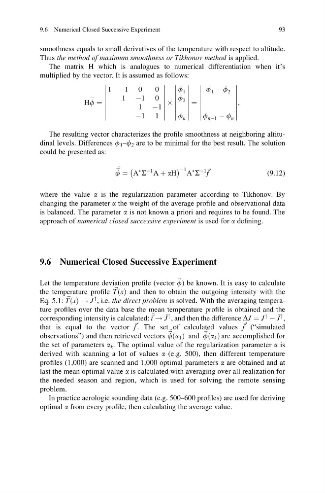
The matrix H which is analogues to numerical differentiation when it’s
multiplied by the vector. It is assumed as follows:
Hf
* ¼
1 À1 0
0
1 À1 0
1 À1
À1 1
Â
f 1
f 2
f n
¼
f 1 À f 2
f nÀ1 À f n
;
The resulting vector characterizes the profile smoothness at neighboring altitudinal levels. Differences f 1 –f 2 are to be minimal for the best result. The solution
could be presented as:
^
~ f ¼ A
Ã
S
À1 A þ aH
À
Á À1 A
Ã
S
À1 ~ f
(9.12)
where the value a is the regularization parameter according to Tikhonov. By
changing the parameter a the weight of the average profile and observational data
is balanced. The parameter a is not known a priori and requires to be found. The
approach of numerical closed successive experiment is used for a defining.
9.6 Numerical Closed Successive Experiment
Let the temperature deviation profile (vector ~ f) be known. It is easy to calculate
the temperature profile ~
TðxÞ and then to obtain the outgoing intensity with the
Eq. 5.1: ~
TðxÞ ! J
" , i.e. the direct problem is solved. With the averaging temperature profiles over the data base the mean temperature profile is obtained and the
corresponding intensity is calculated:
~ t !
J
" , and then the difference DJ ¼ J
"
À
J
" ,
that is equal to the vector ~ f . The set of calculated values ~ f (“simulated
observations”) and then retrieved vectors
^
~ fða 1 Þ and
^
~ fða k Þ are accomplished for
the set of parameters a k . The optimal value of the regularization parameter a is
derived with scanning a lot of values a (e.g. 500), then different temperature
profiles (1,000) are scanned and 1,000 optimal parameters a are obtained and at
last the mean optimal value a is calculated with averaging over all realization for
the needed season and region, which is used for solving the remote sensing
problem.
In practice aerologic sounding data (e.g. 500–600 profiles) are used for deriving
optimal a from every profile, then calculating the average value.
9.6 Numerical Closed Successive Experiment
93
Thus the method of maximum smoothness or Tikhonov method is applied.
The matrix H which is analogues to numerical differentiation when it’s
multiplied by the vector. It is assumed as follows:
Hf
* ¼
1 À1 0
0
1 À1 0
1 À1
À1 1
Â
f 1
f 2
f n
¼
f 1 À f 2
f nÀ1 À f n
;
The resulting vector characterizes the profile smoothness at neighboring altitudinal levels. Differences f 1 –f 2 are to be minimal for the best result. The solution
could be presented as:
^
~ f ¼ A
Ã
S
À1 A þ aH
À
Á À1 A
Ã
S
À1 ~ f
(9.12)
where the value a is the regularization parameter according to Tikhonov. By
changing the parameter a the weight of the average profile and observational data
is balanced. The parameter a is not known a priori and requires to be found. The
approach of numerical closed successive experiment is used for a defining.
9.6 Numerical Closed Successive Experiment
Let the temperature deviation profile (vector ~ f) be known. It is easy to calculate
the temperature profile ~
TðxÞ and then to obtain the outgoing intensity with the
Eq. 5.1: ~
TðxÞ ! J
" , i.e. the direct problem is solved. With the averaging temperature profiles over the data base the mean temperature profile is obtained and the
corresponding intensity is calculated:
~ t !
J
" , and then the difference DJ ¼ J
"
À
J
" ,
that is equal to the vector ~ f . The set of calculated values ~ f (“simulated
observations”) and then retrieved vectors
^
~ fða 1 Þ and
^
~ fða k Þ are accomplished for
the set of parameters a k . The optimal value of the regularization parameter a is
derived with scanning a lot of values a (e.g. 500), then different temperature
profiles (1,000) are scanned and 1,000 optimal parameters a are obtained and at
last the mean optimal value a is calculated with averaging over all realization for
the needed season and region, which is used for solving the remote sensing
problem.
In practice aerologic sounding data (e.g. 500–600 profiles) are used for deriving
optimal a from every profile, then calculating the average value.
9.6 Numerical Closed Successive Experiment
93