

Ri
v
112
6. Spatial Fisheries Model
Mi
TOTALM
V
J
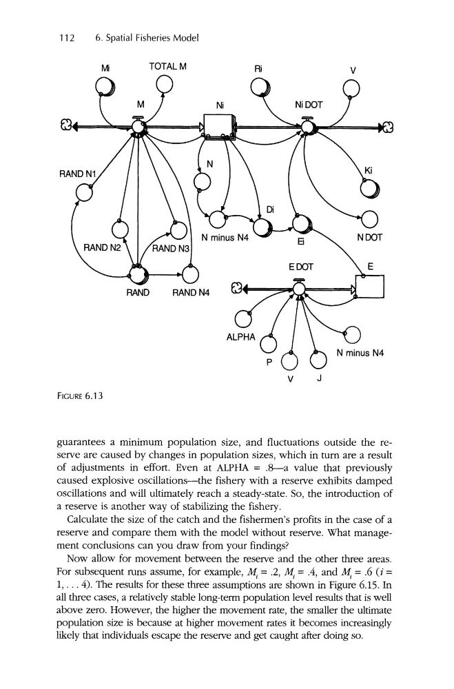
FIGURE 6.13
guarantees a minimu m population size, and fluctuations outside the reserve are cause d by changes in population sizes , which in turn are a result
of adjustments in effort. Even at ALPHA = .8--a value that previously
caused explosive oscillations-the fishery with a reserve exhibits damped
oscillations and will ultimately reach a steady-state. So, the introduc tion of
a reserve is another way of stabilizing the fishery .
Calculate the size of the catch and the fishermen 's profits in the case of a
reserve and compare them with the model without reserve. What management conclusions can you draw from your findings?
Now allow for movement betwee n the reserve and the other three areas.
For subsequent runs assume, for example, M . = .2, M . = .4, and M . = .6 (i =
I
I
I
1, . . . 4). The results for these three assumptions are shown in Figure 6.15. In
all three cases, a relatively stable long-term population level results that is well
above zero. However, the higher the movement rate, the smaller the ultimate
pop ulation size is because at higher movement rates it becomes increasingly
likely that individuals escape the reserve and get caught after doing so.
v
112
6. Spatial Fisheries Model
Mi
TOTALM
V
J
FIGURE 6.13
guarantees a minimu m population size, and fluctuations outside the reserve are cause d by changes in population sizes , which in turn are a result
of adjustments in effort. Even at ALPHA = .8--a value that previously
caused explosive oscillations-the fishery with a reserve exhibits damped
oscillations and will ultimately reach a steady-state. So, the introduc tion of
a reserve is another way of stabilizing the fishery .
Calculate the size of the catch and the fishermen 's profits in the case of a
reserve and compare them with the model without reserve. What management conclusions can you draw from your findings?
Now allow for movement betwee n the reserve and the other three areas.
For subsequent runs assume, for example, M . = .2, M . = .4, and M . = .6 (i =
I
I
I
1, . . . 4). The results for these three assumptions are shown in Figure 6.15. In
all three cases, a relatively stable long-term population level results that is well
above zero. However, the higher the movement rate, the smaller the ultimate
pop ulation size is because at higher movement rates it becomes increasingly
likely that individuals escape the reserve and get caught after doing so.