

6.2. Basic Model with Spatial Movement
1: N v. N DOT
109
180000.00
N
o
T
o
-180000.00
36000.00
N
0.00
72000.00
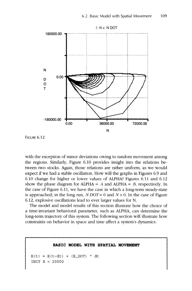
FIGURE 6.12
with the exception of minor deviations owing to random movement among
the regions. Similarly, Figure 6.10 provides insight into the relations between two stocks . Again, those relations are rather uniform, as we would
expect if we had a stable oscillation. How will the graphs in Figures 6.9 and
6.10 change for higher or lower values of ALPHA? Figures 6.11 and 6.12
show the phase diagram for ALPHA = .4 and ALPHA = .8, respectively . In
the case of Figure 6.11, we have the case in which a long-term steady-state
is approached; in the long run , N DOT= 0 and N> O. In the case of Figure
6.12, explosive oscillations lead to ever larger values for N.
The model and model results of this section illustrate how the choice of
a time-invariant behavioral parameter, such as ALPHA, can determine the
long-term trajectory of this system. The following section will illustrate how
constraints on behavior in space and time affect a system's dynamics .
BASIC MODEL WITH SPATIAL MOVEMENT
E(t)
E(t-dt) + (E_DOT) * dt
INIT E = 20000
1: N v. N DOT
109
180000.00
N
o
T
o
-180000.00
36000.00
N
0.00
72000.00
FIGURE 6.12
with the exception of minor deviations owing to random movement among
the regions. Similarly, Figure 6.10 provides insight into the relations between two stocks . Again, those relations are rather uniform, as we would
expect if we had a stable oscillation. How will the graphs in Figures 6.9 and
6.10 change for higher or lower values of ALPHA? Figures 6.11 and 6.12
show the phase diagram for ALPHA = .4 and ALPHA = .8, respectively . In
the case of Figure 6.11, we have the case in which a long-term steady-state
is approached; in the long run , N DOT= 0 and N> O. In the case of Figure
6.12, explosive oscillations lead to ever larger values for N.
The model and model results of this section illustrate how the choice of
a time-invariant behavioral parameter, such as ALPHA, can determine the
long-term trajectory of this system. The following section will illustrate how
constraints on behavior in space and time affect a system's dynamics .
BASIC MODEL WITH SPATIAL MOVEMENT
E(t)
E(t-dt) + (E_DOT) * dt
INIT E = 20000