

106
6. Spatial Fisheries Model
1
\. \ \. \. \ \ \. \ \
0.00
250.00
I
I
j\. \. \. \.
I
"1\. \. \ \.
500.00
750.00
1000.00
Time
1: 150000.00
1: E
1: 300000.00
1:
0.00
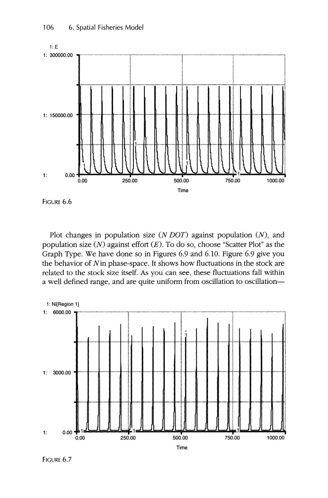
FIGURE 6.6
Plot changes in popul ation size (N D OT) against popul ation (N), and
population size (N) against effort (E ). To do so, choose "Scatter Plot" as the
Graph Type. We have done so in Figures 6.9 and 6.10. Figure 6.9 give you
the behavior of N in phase-space. It shows how fluctuations in the stock are
related to the stock size itself. As you can see, these fluctuations fall within
a we ll defined range, and are quite uniform from oscillation to oscillation1: Ni[Region 1]
1: 6000.00
1: 3000.00
1000.00
1
750.00
0.00 . 1
0.00
1
250.00
500.00
Time
1:
FIGURE 6.7
6. Spatial Fisheries Model
1
\. \ \. \. \ \ \. \ \
0.00
250.00
I
I
j\. \. \. \.
I
"1\. \. \ \.
500.00
750.00
1000.00
Time
1: 150000.00
1: E
1: 300000.00
1:
0.00
FIGURE 6.6
Plot changes in popul ation size (N D OT) against popul ation (N), and
population size (N) against effort (E ). To do so, choose "Scatter Plot" as the
Graph Type. We have done so in Figures 6.9 and 6.10. Figure 6.9 give you
the behavior of N in phase-space. It shows how fluctuations in the stock are
related to the stock size itself. As you can see, these fluctuations fall within
a we ll defined range, and are quite uniform from oscillation to oscillation1: Ni[Region 1]
1: 6000.00
1: 3000.00
1000.00
1
750.00
0.00 . 1
0.00
1
250.00
500.00
Time
1:
FIGURE 6.7