

forest could have multiple returns after hitting leaves and branches of trees,
underlying shrubs, and then the ground.
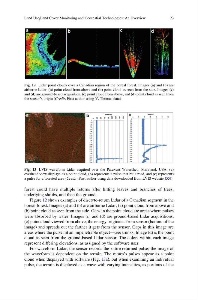
Figure 12 shows examples of discrete-return Lidar of a Canadian segment in the
boreal forest. Images (a) and (b) are airborne Lidar, (a) point cloud from above and
(b) point cloud as seen from the side. Gaps in the point cloud are areas where pulses
were absorbed by water. Images (c) and (d) are ground-based Lidar acquisitions,
(c) point cloud viewed from above, the energy originates from sensor (bottom of the
image) and spreads out the farther it gets from the sensor. Gaps in this image are
areas where the pulse hit an impenetrable object—tree trunks. Image (d) is the point
cloud as seen from the ground-based Lidar sensor. The colors within each image
represent differing elevations, as assigned by the software user.
For waveform Lidar, the sensor records the entire returned pulse; the image of
the waveform is dependent on the terrain. The return’s pulses appear as a point
cloud when displayed with software (Fig. 13a), but when examining an individual
pulse, the terrain is displayed as a wave with varying intensities, as portions of the
Fig. 12 Lidar point clouds over a Canadian region of the boreal forest. Images (a) and (b) are
airborne Lidar, (a) point cloud from above and (b) point cloud as seen from the side. Images (c)
and (d) are ground-based acquisition, (c) point cloud from above, and (d) point cloud as seen from
the sensor’s origin (Credit: First author using V. Thomas data)
Fig. 13 LVIS waveform Lidar acquired over the Patuxent Watershed, Maryland, USA, (a)
overhead view displays as a point cloud, (b) represents a pulse that hit a road, and (c) represents
a pulse for a forested area (Credit: First author using data downloaded from LVIS website [55])
Land Use/Land Cover Monitoring and Geospatial Technologies: An Overview
23
underlying shrubs, and then the ground.
Figure 12 shows examples of discrete-return Lidar of a Canadian segment in the
boreal forest. Images (a) and (b) are airborne Lidar, (a) point cloud from above and
(b) point cloud as seen from the side. Gaps in the point cloud are areas where pulses
were absorbed by water. Images (c) and (d) are ground-based Lidar acquisitions,
(c) point cloud viewed from above, the energy originates from sensor (bottom of the
image) and spreads out the farther it gets from the sensor. Gaps in this image are
areas where the pulse hit an impenetrable object—tree trunks. Image (d) is the point
cloud as seen from the ground-based Lidar sensor. The colors within each image
represent differing elevations, as assigned by the software user.
For waveform Lidar, the sensor records the entire returned pulse; the image of
the waveform is dependent on the terrain. The return’s pulses appear as a point
cloud when displayed with software (Fig. 13a), but when examining an individual
pulse, the terrain is displayed as a wave with varying intensities, as portions of the
Fig. 12 Lidar point clouds over a Canadian region of the boreal forest. Images (a) and (b) are
airborne Lidar, (a) point cloud from above and (b) point cloud as seen from the side. Images (c)
and (d) are ground-based acquisition, (c) point cloud from above, and (d) point cloud as seen from
the sensor’s origin (Credit: First author using V. Thomas data)
Fig. 13 LVIS waveform Lidar acquired over the Patuxent Watershed, Maryland, USA, (a)
overhead view displays as a point cloud, (b) represents a pulse that hit a road, and (c) represents
a pulse for a forested area (Credit: First author using data downloaded from LVIS website [55])
Land Use/Land Cover Monitoring and Geospatial Technologies: An Overview
23