

Identifying Soil and Transport Properties Using a Model
25
Invoking ergodic arguments, we assume that the spatial average of the
concentration over the horizontal plane, C(t,z), can be replaced by, (C) the
ensemble average of concentration over the distributions of the chosen random
parameters. Solute concentration measurements represent average values over a
finite vertical sample length. Where the vertical concentration changes
significantly within the sampling segment, average concentrations may differ
significantly from local concentrations. This is the case where concentration
gradients can change quite significantly within the 20-cm-Iong homogenized core
segments. We therefore compute the ensemble depth-averaged concentration,
which is denoted by [( C (z}, Z2, t»]. Calculating the ensemble mean concentration
and integrating the latter over depth from Zl to Z2 leads to the following result:
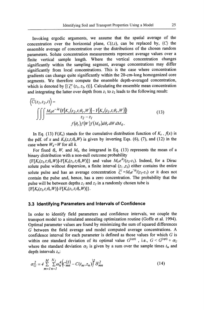
(C(Zj,Zbt)) =
fff
Moe-JJ (F[Ks(Zbt;On W )]- F[K,(z],t;On W )])
Z2 -z]
(13)
f(Or )f(W )f(M 0 )dor dW dM 0 .
In Eq. (13) F(Ks) stands for the cumulative distribution function of Ks ,f{x) is
the pdf. of x and Ks(z,t;O"W) is given by inverting Eqs. (6), (7), and (12) in the
case where Wk = W for all k.
For fixed On W, and Mo, the integrand in Eq. (13) represents the mean of a
binary distribution with a non-null outcome probability
{F[K,(zz,t;O"W)]-F[K,(ZI,t;O"W)]} and value MoeAJ/(zZ-zl)' Indeed, for a Dirac
solute pulse without dispersion, a finite interval (Zl ,zz) either contains the entire
solute pulse and has an average concentration C =Moe-J,.I/(z2-ZI) or it does not
contain the pulse and, hence, has a zero concentration. The probability that the
pulse will be between depths Z/ and Z2 in a randomly chosen tube is
{F[ K,(Z2' t; 0" W)]-F[ KsCZI' t; On W)]}.
3.3 Identifying Parameters and Intervals of Confidence
In order to identify field parameters and confidence intervals, we couple the
transport model to a simulated annealing optimization routine (Goffe et al. 1994).
Optimal parameter values are found by minimizing the sum of squared differences
G between the field average and model computed average concentrations. A
confidence interval for each parameter is defined as those values for which G is
within one standard deviation of its optimal value dopt) , i.e., G < G(opt) + O'G
where the standard deviation O'G is given by a sum over the sample times tm and
depth intervals Zn:
(14)
25
Invoking ergodic arguments, we assume that the spatial average of the
concentration over the horizontal plane, C(t,z), can be replaced by, (C) the
ensemble average of concentration over the distributions of the chosen random
parameters. Solute concentration measurements represent average values over a
finite vertical sample length. Where the vertical concentration changes
significantly within the sampling segment, average concentrations may differ
significantly from local concentrations. This is the case where concentration
gradients can change quite significantly within the 20-cm-Iong homogenized core
segments. We therefore compute the ensemble depth-averaged concentration,
which is denoted by [( C (z}, Z2, t»]. Calculating the ensemble mean concentration
and integrating the latter over depth from Zl to Z2 leads to the following result:
(C(Zj,Zbt)) =
fff
Moe-JJ (F[Ks(Zbt;On W )]- F[K,(z],t;On W )])
Z2 -z]
(13)
f(Or )f(W )f(M 0 )dor dW dM 0 .
In Eq. (13) F(Ks) stands for the cumulative distribution function of Ks ,f{x) is
the pdf. of x and Ks(z,t;O"W) is given by inverting Eqs. (6), (7), and (12) in the
case where Wk = W for all k.
For fixed On W, and Mo, the integrand in Eq. (13) represents the mean of a
binary distribution with a non-null outcome probability
{F[K,(zz,t;O"W)]-F[K,(ZI,t;O"W)]} and value MoeAJ/(zZ-zl)' Indeed, for a Dirac
solute pulse without dispersion, a finite interval (Zl ,zz) either contains the entire
solute pulse and has an average concentration C =Moe-J,.I/(z2-ZI) or it does not
contain the pulse and, hence, has a zero concentration. The probability that the
pulse will be between depths Z/ and Z2 in a randomly chosen tube is
{F[ K,(Z2' t; 0" W)]-F[ KsCZI' t; On W)]}.
3.3 Identifying Parameters and Intervals of Confidence
In order to identify field parameters and confidence intervals, we couple the
transport model to a simulated annealing optimization routine (Goffe et al. 1994).
Optimal parameter values are found by minimizing the sum of squared differences
G between the field average and model computed average concentrations. A
confidence interval for each parameter is defined as those values for which G is
within one standard deviation of its optimal value dopt) , i.e., G < G(opt) + O'G
where the standard deviation O'G is given by a sum over the sample times tm and
depth intervals Zn:
(14)