

110
Water In Ecosystems: A Non Renewable Resource
\ . .•. . •
•..
·o ~--~--~--~~--~~~--~ u --~ ~
z
·.~----~----~--~----~----~ u
h
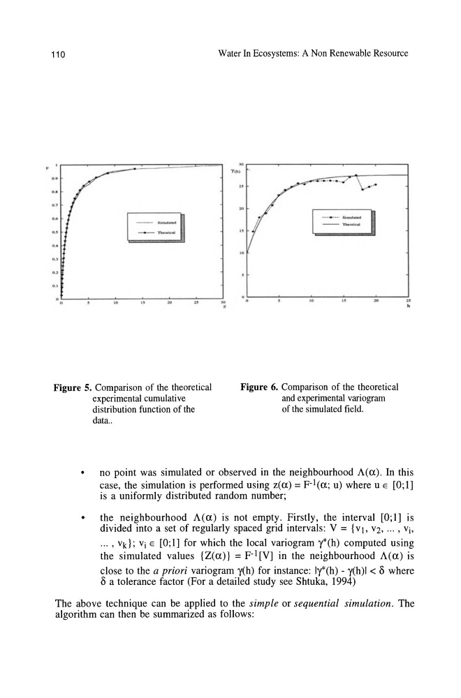
Figure 5. Comparison of the theoretical
experimental cumulative
distribution function of the
data ..
Figure 6. Comparison of the theoretical
and experimental variogram
of the simulated field.
•
no point was simulated or observed in the neighbourhood A(a). In this
case, the simulation is performed using z(a) = F-i(a; u) where u E [0;1]
is a uniformly distributed random number;
•
the neighbourhood A (a) is not empty . Firstly, the interval [0; 1] is
divided into a set of regularly spaced grid intervals: V = {Vi, v2, ... , vi,
... , Vk}; vi E [0;1] for which the local variogram y*(h) computed using
the simulated values {Z( a)} = F-i [V] in the neighbourhood A( a) is
close to the a priori variogram y(h) for instance: Iy*(h) - y(h)1 < () where
() a tolerance factor (For a detailed study see Shtuka, 1994)
The above technique can be applied to the simple or sequential simulation. The
algorithm can then be summarized as follows:
Water In Ecosystems: A Non Renewable Resource
\ . .•. . •
•..
·o ~--~--~--~~--~~~--~ u --~ ~
z
·.~----~----~--~----~----~ u
h
Figure 5. Comparison of the theoretical
experimental cumulative
distribution function of the
data ..
Figure 6. Comparison of the theoretical
and experimental variogram
of the simulated field.
•
no point was simulated or observed in the neighbourhood A(a). In this
case, the simulation is performed using z(a) = F-i(a; u) where u E [0;1]
is a uniformly distributed random number;
•
the neighbourhood A (a) is not empty . Firstly, the interval [0; 1] is
divided into a set of regularly spaced grid intervals: V = {Vi, v2, ... , vi,
... , Vk}; vi E [0;1] for which the local variogram y*(h) computed using
the simulated values {Z( a)} = F-i [V] in the neighbourhood A( a) is
close to the a priori variogram y(h) for instance: Iy*(h) - y(h)1 < () where
() a tolerance factor (For a detailed study see Shtuka, 1994)
The above technique can be applied to the simple or sequential simulation. The
algorithm can then be summarized as follows: