

(1a)
10. Acoustic Models of Sound Production
411
sible acoustical model of the dolphin's tissues from the available data; (2)
utilizing the reversibility of wave propagation to let the model tell us what
its focal characteristics are; and (3) applying the resulting focal information
in forward simulations to determine the emission properties for each
model. Each step of this procedure has yielded new insights into the
acoustic mechanisms of delphinid biosonar.
In order to study the patterns of sound propagation within the forehead
tissues, propagation through tissue models was simulated by numerical integration of the acoustic wave equation. Shear wave velocities for soft tissues
remain less than 1% of the compressional wave sound speed for frequencies below 1MHz, and soft tissue shear wave attenuation coefficients are of
the order of 10
4 times the compressional wave attenuation coefficients
(Frizzell et aI., 1976; Carstensen 1979; Madsen, et aI., 1983). Additionally,
the fact that air sacs normally cover much of the skull surface in the vicinity of the nasal passages in delphinids also suggests that shear modes do not
play a significant role in biosonar emissions. In the current simulations,
tissues (including bone) were modeled as inhomogeneous fluids and shear
wave modes were ignored.
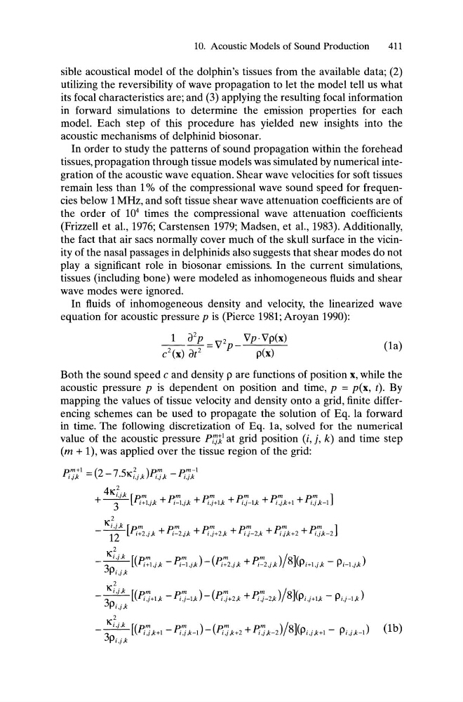
In fluids of inhomogeneous density and velocity, the linearized wave
equation for acoustic pressure p is (Pierce 1981; Aroyan 1990):
_1_ "(Pp = V 2p_ Vp· Vp(x)
c
2 (x) ot
2
p(x)
Both the sound speed c and density P are functions of position x, while the
acoustic pressure p is dependent on position and time, p = p(x, t). By
mapping the values of tissue velocity and density onto a grid, finite differencing schemes can be used to propagate the solution of Eq. la forward
in time. The following discretization of Eq. la, solved for the numerical
value of the acoustic pressure Pt'j,i/ at grid position (i, j, k) and time step
(m + 1), was applied over the tissue region of the grid:
pm,k+l = (2 -7.51(2,k}p m ,k - pm,k-I
lJ
I,]
I,]
l,J
41(;'j,k [pm
pm
pm
pm
pm
pm]
+-3- i+l,j,k + i-I,j,k + i,j+l,k + i,j-I,k + i,j,k+1 + i,j,k-I
2
1(i,j,k [pm
pm
pm
pm
pm
pm]
- U i+2,j,k + i-2j,k + i,j+2,k + ij-2,k + ij,k+2 + i,j,k-2
2
- 31(i,j,k [(P;:I.j,k -P;'::I,j,k)-(P;72,j,k +P;'::2,j,k)/8](Pi+l,j,k - PHj,k)
Pi,j,k
1(2
-~[(P;J+I,k-P;J-I,k}-(P;J+2,k +P;J-2,k}/8](Pi,j+I,k - Pi,j-I,k)
Pi,j,k
1(2
- - 3
" /,k [(P;J,k+1 -P;J,k-I)-(P;J,k+2 +P;J,k-2)/8](Pi,j,k+1 - Pi,j,k-l) (1b)
Pi,j,k
10. Acoustic Models of Sound Production
411
sible acoustical model of the dolphin's tissues from the available data; (2)
utilizing the reversibility of wave propagation to let the model tell us what
its focal characteristics are; and (3) applying the resulting focal information
in forward simulations to determine the emission properties for each
model. Each step of this procedure has yielded new insights into the
acoustic mechanisms of delphinid biosonar.
In order to study the patterns of sound propagation within the forehead
tissues, propagation through tissue models was simulated by numerical integration of the acoustic wave equation. Shear wave velocities for soft tissues
remain less than 1% of the compressional wave sound speed for frequencies below 1MHz, and soft tissue shear wave attenuation coefficients are of
the order of 10
4 times the compressional wave attenuation coefficients
(Frizzell et aI., 1976; Carstensen 1979; Madsen, et aI., 1983). Additionally,
the fact that air sacs normally cover much of the skull surface in the vicinity of the nasal passages in delphinids also suggests that shear modes do not
play a significant role in biosonar emissions. In the current simulations,
tissues (including bone) were modeled as inhomogeneous fluids and shear
wave modes were ignored.
In fluids of inhomogeneous density and velocity, the linearized wave
equation for acoustic pressure p is (Pierce 1981; Aroyan 1990):
_1_ "(Pp = V 2p_ Vp· Vp(x)
c
2 (x) ot
2
p(x)
Both the sound speed c and density P are functions of position x, while the
acoustic pressure p is dependent on position and time, p = p(x, t). By
mapping the values of tissue velocity and density onto a grid, finite differencing schemes can be used to propagate the solution of Eq. la forward
in time. The following discretization of Eq. la, solved for the numerical
value of the acoustic pressure Pt'j,i/ at grid position (i, j, k) and time step
(m + 1), was applied over the tissue region of the grid:
pm,k+l = (2 -7.51(2,k}p m ,k - pm,k-I
lJ
I,]
I,]
l,J
41(;'j,k [pm
pm
pm
pm
pm
pm]
+-3- i+l,j,k + i-I,j,k + i,j+l,k + i,j-I,k + i,j,k+1 + i,j,k-I
2
1(i,j,k [pm
pm
pm
pm
pm
pm]
- U i+2,j,k + i-2j,k + i,j+2,k + ij-2,k + ij,k+2 + i,j,k-2
2
- 31(i,j,k [(P;:I.j,k -P;'::I,j,k)-(P;72,j,k +P;'::2,j,k)/8](Pi+l,j,k - PHj,k)
Pi,j,k
1(2
-~[(P;J+I,k-P;J-I,k}-(P;J+2,k +P;J-2,k}/8](Pi,j+I,k - Pi,j-I,k)
Pi,j,k
1(2
- - 3
" /,k [(P;J,k+1 -P;J,k-I)-(P;J,k+2 +P;J,k-2)/8](Pi,j,k+1 - Pi,j,k-l) (1b)
Pi,j,k