

A Loading Criterion for the Feasibility of Biomanipulation
147
1.0 ~---------------r--~~
c...
0.8
-...l
11)
.......
..... ,
~ "0
I..,
bO-;0.6
c:: I..,
~
11)
.....
. -
..9 -
u ~ 0.4
.....
bll
I..,
.... ~
11)
E
........
' - '
::1
- 0.2
0
:>
0.0
0
0.01
0.02
0.03
0.04
Dilution rate D (d - I )
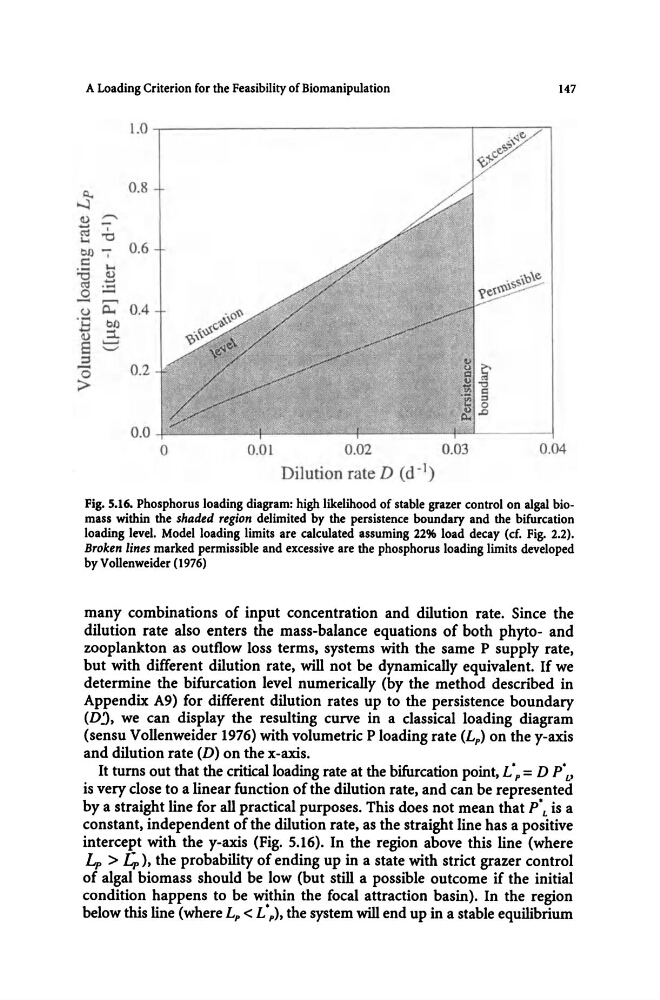
Fig. 5.16. Phosphorus loading diagram: high likelihood of stable grazer control on algal biomass within the shaded region delimited by the persistence boundary and the bifurcation
loading level. Model loading limits are calculated assuming 22% load decay (cf. Fig. 2.2).
Broken lines marked permissible and excessive are the phosphorus loading limits developed
by Vollenweider (1976)
many combinations of input concentration and dilution rate. Since the
dilution rate also enters the mass-balance equations of both phyto- and
zooplankton as outflow loss terms, systems with the same P supply rate,
but with different dilution rate, will not be dynamically equivalent. If we
determine the bifurcation level numerically (by the method described in
Appendix A9) for different dilution rates up to the persistence boundary
(Dj, we can display the resulting curve in a classical loading diagram
(sensu Vollenweider 1976) with volumetric P loading rate (Lp) on the y-axis
and dilution rate (D) on the x-axis.
It turns out that the critical loading rate at the bifurcation point, L·p = D p· v
is very close to a linear function of the dilution rate, and can be represented
by a straight line for all practical purposes. This does not mean that p· L is a
constant, independent of the dilution rate, as the straight line has a positive
intercept with the y-axis (Fig. 5.16). In the region above this line (where
4 > "£P), the probability of ending up in a state with strict grazer control
of algal biomass should be low (but still a possible outcome if the initial
condition happens to be within the focal attraction basin). In the region
below this line (where Lp < L·p), the system will end up in a stable equilibrium
147
1.0 ~---------------r--~~
c...
0.8
-...l
11)
.......
..... ,
~ "0
I..,
bO-;0.6
c:: I..,
~
11)
.....
. -
..9 -
u ~ 0.4
.....
bll
I..,
.... ~
11)
E
........
' - '
::1
- 0.2
0
:>
0.0
0
0.01
0.02
0.03
0.04
Dilution rate D (d - I )
Fig. 5.16. Phosphorus loading diagram: high likelihood of stable grazer control on algal biomass within the shaded region delimited by the persistence boundary and the bifurcation
loading level. Model loading limits are calculated assuming 22% load decay (cf. Fig. 2.2).
Broken lines marked permissible and excessive are the phosphorus loading limits developed
by Vollenweider (1976)
many combinations of input concentration and dilution rate. Since the
dilution rate also enters the mass-balance equations of both phyto- and
zooplankton as outflow loss terms, systems with the same P supply rate,
but with different dilution rate, will not be dynamically equivalent. If we
determine the bifurcation level numerically (by the method described in
Appendix A9) for different dilution rates up to the persistence boundary
(Dj, we can display the resulting curve in a classical loading diagram
(sensu Vollenweider 1976) with volumetric P loading rate (Lp) on the y-axis
and dilution rate (D) on the x-axis.
It turns out that the critical loading rate at the bifurcation point, L·p = D p· v
is very close to a linear function of the dilution rate, and can be represented
by a straight line for all practical purposes. This does not mean that p· L is a
constant, independent of the dilution rate, as the straight line has a positive
intercept with the y-axis (Fig. 5.16). In the region above this line (where
4 > "£P), the probability of ending up in a state with strict grazer control
of algal biomass should be low (but still a possible outcome if the initial
condition happens to be within the focal attraction basin). In the region
below this line (where Lp < L·p), the system will end up in a stable equilibrium