

128
Nutrients, Algae and Herbivores - the Paradox of Enrichment Revisited
MacArthur 1963; Tilman 1980). Canale (1970) showed that in a nutrientcontrolled prey-predator system with nutrient conservation, the long-term
dynamics will be confined to a plane, and thus reducible to a system with
only two state variables. As the present model is irreducibly threedimensional due to the non-conservative representation of total phosphorus, the isoclines will be surfaces in (P, C, Z) space, which are much harder
to visualize and analyze graphically.
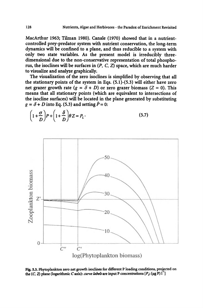
The visualization of the zero isoclines is simplified by observing that all
the stationary points of the system in Eqs. (5.1)-(5.3) will either have zero
net grazer growth rate (g = J + D) or zero grazer biomass (Z = 0). This
means that all stationary points (which are equivalent to intersections of
the isocline surfaces) will be located in the plane generated by substituting
g = J + D into Eq. (5.3) and setting P = 0:
(1 + ~)P+(l+ ~ )OZ= PL·
(5.7)
rJ)
rJ)
~
8
o
.- .0
s:::::
50
40
o z'
~
~E$~'--~
........
0..
o
o
N
20
10
C"
c'
log(Phytoplankton biomass)
Fig. 5.3. Phytoplankton zero net growth isoclines for different P loading conditions, pro!fCted on
the (c. Z) plane (logarithmic C axis): curve klbe/sare input P concentrations [PL: (l1g P) I )
Nutrients, Algae and Herbivores - the Paradox of Enrichment Revisited
MacArthur 1963; Tilman 1980). Canale (1970) showed that in a nutrientcontrolled prey-predator system with nutrient conservation, the long-term
dynamics will be confined to a plane, and thus reducible to a system with
only two state variables. As the present model is irreducibly threedimensional due to the non-conservative representation of total phosphorus, the isoclines will be surfaces in (P, C, Z) space, which are much harder
to visualize and analyze graphically.
The visualization of the zero isoclines is simplified by observing that all
the stationary points of the system in Eqs. (5.1)-(5.3) will either have zero
net grazer growth rate (g = J + D) or zero grazer biomass (Z = 0). This
means that all stationary points (which are equivalent to intersections of
the isocline surfaces) will be located in the plane generated by substituting
g = J + D into Eq. (5.3) and setting P = 0:
(1 + ~)P+(l+ ~ )OZ= PL·
(5.7)
rJ)
rJ)
~
8
o
.- .0
s:::::
50
40
o z'
~
~E$~'--~
........
0..
o
o
N
20
10
C"
c'
log(Phytoplankton biomass)
Fig. 5.3. Phytoplankton zero net growth isoclines for different P loading conditions, pro!fCted on
the (c. Z) plane (logarithmic C axis): curve klbe/sare input P concentrations [PL: (l1g P) I )