

14 Underwater Multimodal Survey: Merging Optical and Acoustic Data
229
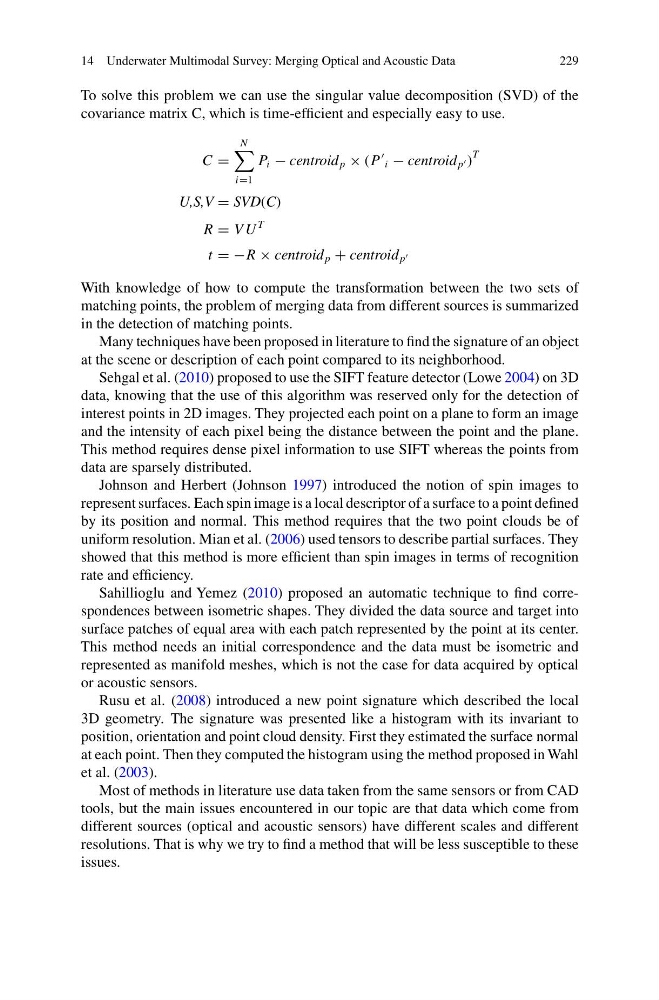
To solve this problem we can use the singular value decomposition (SVD) of the
covariance matrix C, which is time-efficient and especially easy to use.
C =
N
i=1
P i − centroid p × (P
i − centroid p )
T
U,S,V = SVD(C)
R = V U
T
t = −R × centroid p + centroid p
With knowledge of how to compute the transformation between the two sets of
matching points, the problem of merging data from different sources is summarized
in the detection of matching points.
Many techniques have been proposed in literature to find the signature of an object
at the scene or description of each point compared to its neighborhood.
Sehgal et al. (2010) proposed to use the SIFT feature detector (Lowe 2004) on 3D
data, knowing that the use of this algorithm was reserved only for the detection of
interest points in 2D images. They projected each point on a plane to form an image
and the intensity of each pixel being the distance between the point and the plane.
This method requires dense pixel information to use SIFT whereas the points from
data are sparsely distributed.
Johnson and Herbert (Johnson 1997) introduced the notion of spin images to
represent surfaces. Each spin image is a local descriptor of a surface to a point defined
by its position and normal. This method requires that the two point clouds be of
uniform resolution. Mian et al. (2006) used tensors to describe partial surfaces. They
showed that this method is more efficient than spin images in terms of recognition
rate and efficiency.
Sahillioglu and Yemez (2010) proposed an automatic technique to find correspondences between isometric shapes. They divided the data source and target into
surface patches of equal area with each patch represented by the point at its center.
This method needs an initial correspondence and the data must be isometric and
represented as manifold meshes, which is not the case for data acquired by optical
or acoustic sensors.
Rusu et al. (2008) introduced a new point signature which described the local
3D geometry. The signature was presented like a histogram with its invariant to
position, orientation and point cloud density. First they estimated the surface normal
at each point. Then they computed the histogram using the method proposed in Wahl
et al. (2003).
Most of methods in literature use data taken from the same sensors or from CAD
tools, but the main issues encountered in our topic are that data which come from
different sources (optical and acoustic sensors) have different scales and different
resolutions. That is why we try to find a method that will be less susceptible to these
issues.
229
To solve this problem we can use the singular value decomposition (SVD) of the
covariance matrix C, which is time-efficient and especially easy to use.
C =
N
i=1
P i − centroid p × (P
i − centroid p )
T
U,S,V = SVD(C)
R = V U
T
t = −R × centroid p + centroid p
With knowledge of how to compute the transformation between the two sets of
matching points, the problem of merging data from different sources is summarized
in the detection of matching points.
Many techniques have been proposed in literature to find the signature of an object
at the scene or description of each point compared to its neighborhood.
Sehgal et al. (2010) proposed to use the SIFT feature detector (Lowe 2004) on 3D
data, knowing that the use of this algorithm was reserved only for the detection of
interest points in 2D images. They projected each point on a plane to form an image
and the intensity of each pixel being the distance between the point and the plane.
This method requires dense pixel information to use SIFT whereas the points from
data are sparsely distributed.
Johnson and Herbert (Johnson 1997) introduced the notion of spin images to
represent surfaces. Each spin image is a local descriptor of a surface to a point defined
by its position and normal. This method requires that the two point clouds be of
uniform resolution. Mian et al. (2006) used tensors to describe partial surfaces. They
showed that this method is more efficient than spin images in terms of recognition
rate and efficiency.
Sahillioglu and Yemez (2010) proposed an automatic technique to find correspondences between isometric shapes. They divided the data source and target into
surface patches of equal area with each patch represented by the point at its center.
This method needs an initial correspondence and the data must be isometric and
represented as manifold meshes, which is not the case for data acquired by optical
or acoustic sensors.
Rusu et al. (2008) introduced a new point signature which described the local
3D geometry. The signature was presented like a histogram with its invariant to
position, orientation and point cloud density. First they estimated the surface normal
at each point. Then they computed the histogram using the method proposed in Wahl
et al. (2003).
Most of methods in literature use data taken from the same sensors or from CAD
tools, but the main issues encountered in our topic are that data which come from
different sources (optical and acoustic sensors) have different scales and different
resolutions. That is why we try to find a method that will be less susceptible to these
issues.