

196
E. W. Koch, J. D. Ackerman, J. Verduin and M. van Keulen
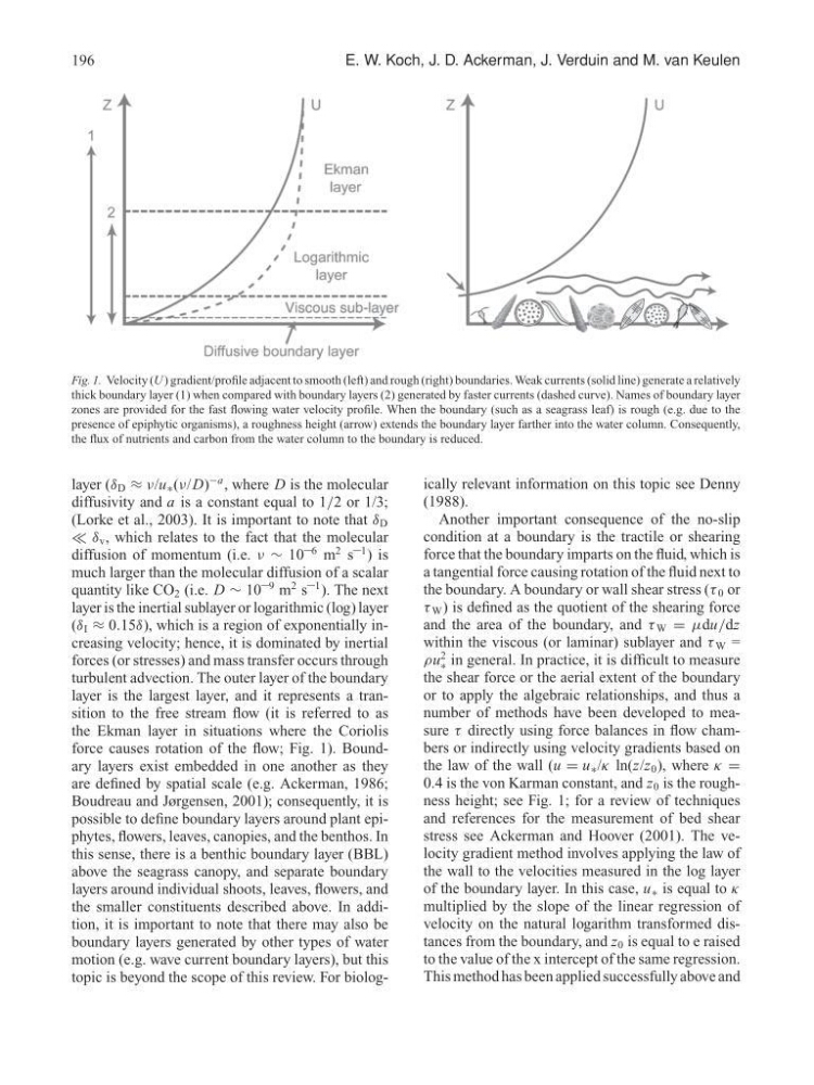
Fig. 1. Velocity (U ) gradient/profile adjacent to smooth (left) and rough (right) boundaries. Weak currents (solid line) generate a relatively
thick boundary layer (1) when compared with boundary layers (2) generated by faster currents (dashed curve). Names of boundary layer
zones are provided for the fast flowing water velocity profile. When the boundary (such as a seagrass leaf) is rough (e.g. due to the
presence of epiphytic organisms), a roughness height (arrow) extends the boundary layer farther into the water column. Consequently,
the flux of nutrients and carbon from the water column to the boundary is reduced.
layer (δ D ≈ ν/u ∗ (ν/D)
−a , where D is the molecular
diffusivity and a is a constant equal to 1/2 or 1/3;
(Lorke et al., 2003). It is important to note that δ D
δ v , which relates to the fact that the molecular
diffusion of momentum (i.e. ν ∼ 10 –6 m
2 s –1 ) is
much larger than the molecular diffusion of a scalar
quantity like CO 2 (i.e. D ∼ 10 –9 m
2 s –1 ). The next
layer is the inertial sublayer or logarithmic (log) layer
(δ I ≈ 0.15δ), which is a region of exponentially increasing velocity; hence, it is dominated by inertial
forces (or stresses) and mass transfer occurs through
turbulent advection. The outer layer of the boundary
layer is the largest layer, and it represents a transition to the free stream flow (it is referred to as
the Ekman layer in situations where the Coriolis
force causes rotation of the flow; Fig. 1). Boundary layers exist embedded in one another as they
are defined by spatial scale (e.g. Ackerman, 1986;
Boudreau and Jørgensen, 2001); consequently, it is
possible to define boundary layers around plant epiphytes, flowers, leaves, canopies, and the benthos. In
this sense, there is a benthic boundary layer (BBL)
above the seagrass canopy, and separate boundary
layers around individual shoots, leaves, flowers, and
the smaller constituents described above. In addition, it is important to note that there may also be
boundary layers generated by other types of water
motion (e.g. wave current boundary layers), but this
topic is beyond the scope of this review. For biologically relevant information on this topic see Denny
(1988).
Another important consequence of the no-slip
condition at a boundary is the tractile or shearing
force that the boundary imparts on the fluid, which is
a tangential force causing rotation of the fluid next to
the boundary. A boundary or wall shear stress (τ 0 or
τ W ) is defined as the quotient of the shearing force
and the area of the boundary, and τ W = µdu/dz
within the viscous (or laminar) sublayer and τ W =
ρu
2
∗ in general. In practice, it is difficult to measure
the shear force or the aerial extent of the boundary
or to apply the algebraic relationships, and thus a
number of methods have been developed to measure τ directly using force balances in flow chambers or indirectly using velocity gradients based on
the law of the wall (u = u ∗ /κ ln(z/z 0 ), where κ =
0.4 is the von Karman constant, and z 0 is the roughness height; see Fig. 1; for a review of techniques
and references for the measurement of bed shear
stress see Ackerman and Hoover (2001). The velocity gradient method involves applying the law of
the wall to the velocities measured in the log layer
of the boundary layer. In this case, u ∗ is equal to κ
multiplied by the slope of the linear regression of
velocity on the natural logarithm transformed distances from the boundary, and z 0 is equal to e raised
to the value of the x intercept of the same regression.
This method has been applied successfully above and
E. W. Koch, J. D. Ackerman, J. Verduin and M. van Keulen
Fig. 1. Velocity (U ) gradient/profile adjacent to smooth (left) and rough (right) boundaries. Weak currents (solid line) generate a relatively
thick boundary layer (1) when compared with boundary layers (2) generated by faster currents (dashed curve). Names of boundary layer
zones are provided for the fast flowing water velocity profile. When the boundary (such as a seagrass leaf) is rough (e.g. due to the
presence of epiphytic organisms), a roughness height (arrow) extends the boundary layer farther into the water column. Consequently,
the flux of nutrients and carbon from the water column to the boundary is reduced.
layer (δ D ≈ ν/u ∗ (ν/D)
−a , where D is the molecular
diffusivity and a is a constant equal to 1/2 or 1/3;
(Lorke et al., 2003). It is important to note that δ D
δ v , which relates to the fact that the molecular
diffusion of momentum (i.e. ν ∼ 10 –6 m
2 s –1 ) is
much larger than the molecular diffusion of a scalar
quantity like CO 2 (i.e. D ∼ 10 –9 m
2 s –1 ). The next
layer is the inertial sublayer or logarithmic (log) layer
(δ I ≈ 0.15δ), which is a region of exponentially increasing velocity; hence, it is dominated by inertial
forces (or stresses) and mass transfer occurs through
turbulent advection. The outer layer of the boundary
layer is the largest layer, and it represents a transition to the free stream flow (it is referred to as
the Ekman layer in situations where the Coriolis
force causes rotation of the flow; Fig. 1). Boundary layers exist embedded in one another as they
are defined by spatial scale (e.g. Ackerman, 1986;
Boudreau and Jørgensen, 2001); consequently, it is
possible to define boundary layers around plant epiphytes, flowers, leaves, canopies, and the benthos. In
this sense, there is a benthic boundary layer (BBL)
above the seagrass canopy, and separate boundary
layers around individual shoots, leaves, flowers, and
the smaller constituents described above. In addition, it is important to note that there may also be
boundary layers generated by other types of water
motion (e.g. wave current boundary layers), but this
topic is beyond the scope of this review. For biologically relevant information on this topic see Denny
(1988).
Another important consequence of the no-slip
condition at a boundary is the tractile or shearing
force that the boundary imparts on the fluid, which is
a tangential force causing rotation of the fluid next to
the boundary. A boundary or wall shear stress (τ 0 or
τ W ) is defined as the quotient of the shearing force
and the area of the boundary, and τ W = µdu/dz
within the viscous (or laminar) sublayer and τ W =
ρu
2
∗ in general. In practice, it is difficult to measure
the shear force or the aerial extent of the boundary
or to apply the algebraic relationships, and thus a
number of methods have been developed to measure τ directly using force balances in flow chambers or indirectly using velocity gradients based on
the law of the wall (u = u ∗ /κ ln(z/z 0 ), where κ =
0.4 is the von Karman constant, and z 0 is the roughness height; see Fig. 1; for a review of techniques
and references for the measurement of bed shear
stress see Ackerman and Hoover (2001). The velocity gradient method involves applying the law of
the wall to the velocities measured in the log layer
of the boundary layer. In this case, u ∗ is equal to κ
multiplied by the slope of the linear regression of
velocity on the natural logarithm transformed distances from the boundary, and z 0 is equal to e raised
to the value of the x intercept of the same regression.
This method has been applied successfully above and