

Production in the Indian Ocean and the Transfer from the Primary to the Secondary Level 481
primary production and 10% of secondary production and using a mean of the two
values. The carbon was raised to wet weight of fish, using the factor 7.47 (VINOGRADOV,
1953), and the quantities were raised to the 5° square by the area factor 6.774 . 10 5 ;
for those squares cut by a coastline, a further area factor was incorporated. Figs. 5 a
and b shows the distribution of tertiary production by half-yearly periods in each
monsoon.
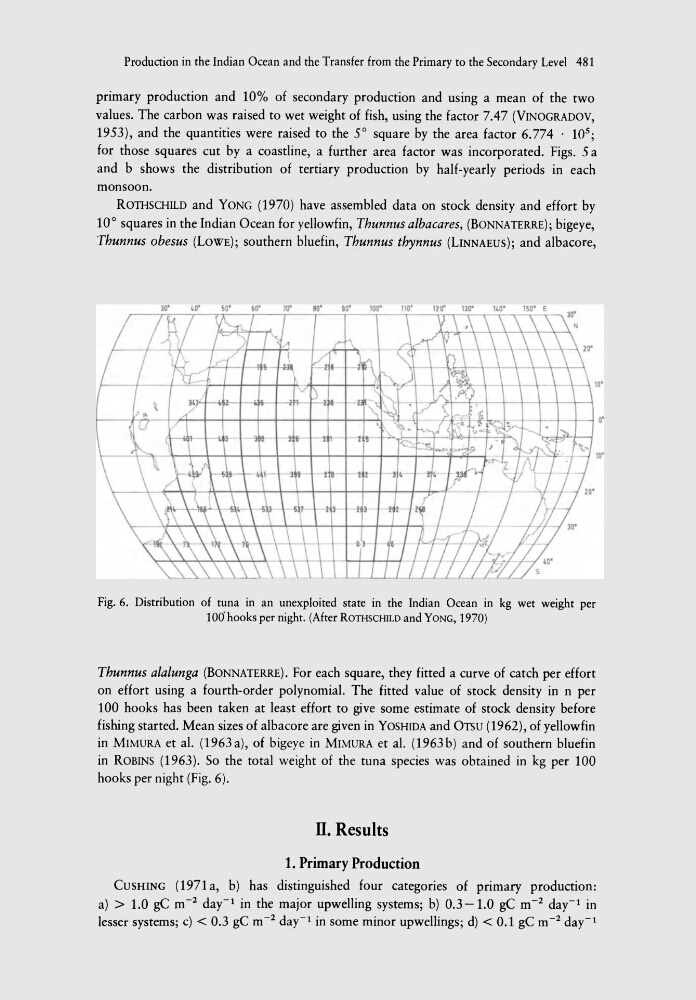
ROTHSCHILD and YONG (1970) have assembled data on stock density and effort by
10° squares in the Indian Ocean for yeIIowfin, Thunnus albacares, (BONNATERRE); bigeye,
Thunnus obesus (LOWE); southern bluefin, Thunnus thynnus (LINNAEUS); and albacore,
UD'
lW E
la'
+--+--+--t---i 0'
la'
Fig. 6. Distribution of tuna in an unexploited state in the Indian Ocean in kg wet weight per
100 hooks per night. (After ROTHSCHILD and YONG, 1970)
Thunnus alalunga (BONNATERRE). For each square, they fitted a curve of catch per effort
on effort using a fourth-order polynomial. The fitted value of stock density in n per
100 hooks has been taken at least effort to give some estimate of stock density before
fishing started. Mean sizes of albacore are given in YOSHIDA and OTSU (1962), of yellowfin
in MIMURA et al. (1963 a), of bigeye in MIMURA et al. (1963 b) and of southern bluefin
in ROBINS (1963). So the total weight of the tuna species was obtained in kg per 100
hooks per night (Fig. 6).
n. Results
1, Primary Production
CUSHING (1971 a, b) has distinguished four categories of primary production:
a) > 1.0 gC m -2 day-l in the major upwelling systems; b) 0.3 -1.0 gC m- 2 day-l in
lesser systems; c) < 0.3 gC m- 2 day-l in some minor upwellings; d) < 0.1 gC m- 2 day-l
primary production and 10% of secondary production and using a mean of the two
values. The carbon was raised to wet weight of fish, using the factor 7.47 (VINOGRADOV,
1953), and the quantities were raised to the 5° square by the area factor 6.774 . 10 5 ;
for those squares cut by a coastline, a further area factor was incorporated. Figs. 5 a
and b shows the distribution of tertiary production by half-yearly periods in each
monsoon.
ROTHSCHILD and YONG (1970) have assembled data on stock density and effort by
10° squares in the Indian Ocean for yeIIowfin, Thunnus albacares, (BONNATERRE); bigeye,
Thunnus obesus (LOWE); southern bluefin, Thunnus thynnus (LINNAEUS); and albacore,
UD'
lW E
la'
+--+--+--t---i 0'
la'
Fig. 6. Distribution of tuna in an unexploited state in the Indian Ocean in kg wet weight per
100 hooks per night. (After ROTHSCHILD and YONG, 1970)
Thunnus alalunga (BONNATERRE). For each square, they fitted a curve of catch per effort
on effort using a fourth-order polynomial. The fitted value of stock density in n per
100 hooks has been taken at least effort to give some estimate of stock density before
fishing started. Mean sizes of albacore are given in YOSHIDA and OTSU (1962), of yellowfin
in MIMURA et al. (1963 a), of bigeye in MIMURA et al. (1963 b) and of southern bluefin
in ROBINS (1963). So the total weight of the tuna species was obtained in kg per 100
hooks per night (Fig. 6).
n. Results
1, Primary Production
CUSHING (1971 a, b) has distinguished four categories of primary production:
a) > 1.0 gC m -2 day-l in the major upwelling systems; b) 0.3 -1.0 gC m- 2 day-l in
lesser systems; c) < 0.3 gC m- 2 day-l in some minor upwellings; d) < 0.1 gC m- 2 day-l