

346
30
25
20
-
'2
g 15
CI:
10
5
o
a)
o
•
•
•
2
4
6
B
Spawner
30
25
20
- '2
g 15
CI:
10
5
o
b)
o
D.G. Chen
•
2
4
6
B
Spawner
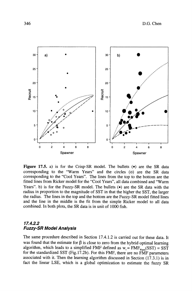
Figure 17.5. a) is for the Crisp-SR model. The bullets (e) are the SR data
corresponding to the "WarmY ears" and the cireles ( 0) are the SR data
corresponding to the "Cool Years". The lines from the top to the bottom are the
fitted lines from Ricker model for the "Cool Years", all data combined and "Warm
Years". b) is for the Fuzzy-SR model. The bullets (e) are the SR data with the
radius in proportion to the magnitude of SST in that the higher the SST, the larger
the radius. The lines in the top and the bottom are the Fuzzy-SR model fitted lines
and the line in the middle is the fit from the simple Ricker model to a11 data
combined. In both plots, the SR data is in unit of 1000 fish.
17.4.2.2
Fuzzy-SR Model Analysis
The same procedure described in Section 17.4.1.2 is carried out for these data. It
was found that the estimate for ß is elose to zero from the hybrid optimallearning
algorithm, which leads to a simplified FMF defined as w, = FMFwann(SST) = SST
for the standardized SST (Fig.17.2b). For this FMF, there are no FMF parameters
associated with it. Then the learning algorithm discussed in Section (17.3.1) is in
fact the linear LSE, which is aglobai optimization to estimate the fuzzy SR
30
25
20
-
'2
g 15
CI:
10
5
o
a)
o
•
•
•
2
4
6
B
Spawner
30
25
20
- '2
g 15
CI:
10
5
o
b)
o
D.G. Chen
•
2
4
6
B
Spawner
Figure 17.5. a) is for the Crisp-SR model. The bullets (e) are the SR data
corresponding to the "WarmY ears" and the cireles ( 0) are the SR data
corresponding to the "Cool Years". The lines from the top to the bottom are the
fitted lines from Ricker model for the "Cool Years", all data combined and "Warm
Years". b) is for the Fuzzy-SR model. The bullets (e) are the SR data with the
radius in proportion to the magnitude of SST in that the higher the SST, the larger
the radius. The lines in the top and the bottom are the Fuzzy-SR model fitted lines
and the line in the middle is the fit from the simple Ricker model to a11 data
combined. In both plots, the SR data is in unit of 1000 fish.
17.4.2.2
Fuzzy-SR Model Analysis
The same procedure described in Section 17.4.1.2 is carried out for these data. It
was found that the estimate for ß is elose to zero from the hybrid optimallearning
algorithm, which leads to a simplified FMF defined as w, = FMFwann(SST) = SST
for the standardized SST (Fig.17.2b). For this FMF, there are no FMF parameters
associated with it. Then the learning algorithm discussed in Section (17.3.1) is in
fact the linear LSE, which is aglobai optimization to estimate the fuzzy SR