

344
D.G. ehen
17.4.1.3
Bootstrap Re-sampling Analysis
The residuals from the Fuzzy-SR model are diagnosed for the independence and
homogeneity. The independence for the residuals can be checked by the time
series autocorrelation function (Box et. al. 1994) and the homogeneity of residuals
can be identified from the residual plot and also the Kolmogorov0.5
1.0
1.5
2.0
0.015 0.020 0.025 0.030 0.035 0.040 0 .04~
Ricker a in Cool Regime
Ricker b in Cool Regime
~ 1.0
~ 40
'(j) 0.8
'(j) 30
I
"I~II
1
~!i~ ~~~
~ 0.8
'(j) 0.6
5i 0.4
Cl 0.2
0.0
0.5
1.0
1.5
Ricker a in Warm Regime
1.0
1
0.0 L.;:::::"J1!::::::==::::!:::;==;:!L--=::::~
·0.5
0.0
0.5
1.0
1.5
2.0
Ricker a1-a2
0.03 0.04 0.05 0.06 0.07 0.08 0.09
Ricker b in Warm Regime
.?:- 30 1
.~ 20
~ ~ L=~~~~===~=~~~~~
·0.06
-0.04
·0.02
0.0
Ricker b1-b2
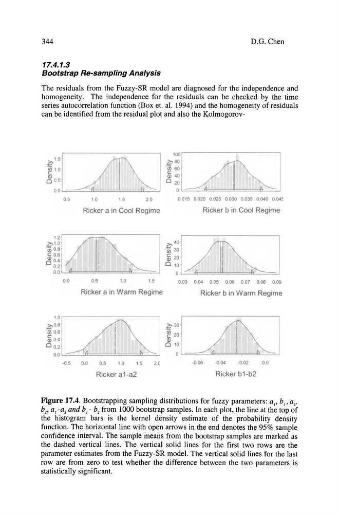
Figure 17.4. Bootstrapping sampling distributions for fuzzy parameters: a p b" a 2 ,
b 2 , a,-a 2 and b, - b 2 from 1000 bootstrap sampies. In each plot, the line at the top of
the histogram bars is the kernel density estimate of the probability density
function. The horizontalline with open arrows in the end denotes the 95% sample
confidence interval. The sampie means from the boots trap sampies are marked as
the dashed vertical lines. The vertical solid lines für the first two rows are the
parameter estimates from the Fuzzy-SR model. The vertical solid lines for the last
row are from zero to test whether the difference between the two parameters is
statistically significant.
D.G. ehen
17.4.1.3
Bootstrap Re-sampling Analysis
The residuals from the Fuzzy-SR model are diagnosed for the independence and
homogeneity. The independence for the residuals can be checked by the time
series autocorrelation function (Box et. al. 1994) and the homogeneity of residuals
can be identified from the residual plot and also the Kolmogorov0.5
1.0
1.5
2.0
0.015 0.020 0.025 0.030 0.035 0.040 0 .04~
Ricker a in Cool Regime
Ricker b in Cool Regime
~ 1.0
~ 40
'(j) 0.8
'(j) 30
I
"I~II
1
~!i~ ~~~
~ 0.8
'(j) 0.6
5i 0.4
Cl 0.2
0.0
0.5
1.0
1.5
Ricker a in Warm Regime
1.0
1
0.0 L.;:::::"J1!::::::==::::!:::;==;:!L--=::::~
·0.5
0.0
0.5
1.0
1.5
2.0
Ricker a1-a2
0.03 0.04 0.05 0.06 0.07 0.08 0.09
Ricker b in Warm Regime
.?:- 30 1
.~ 20
~ ~ L=~~~~===~=~~~~~
·0.06
-0.04
·0.02
0.0
Ricker b1-b2
Figure 17.4. Bootstrapping sampling distributions for fuzzy parameters: a p b" a 2 ,
b 2 , a,-a 2 and b, - b 2 from 1000 bootstrap sampies. In each plot, the line at the top of
the histogram bars is the kernel density estimate of the probability density
function. The horizontalline with open arrows in the end denotes the 95% sample
confidence interval. The sampie means from the boots trap sampies are marked as
the dashed vertical lines. The vertical solid lines für the first two rows are the
parameter estimates from the Fuzzy-SR model. The vertical solid lines for the last
row are from zero to test whether the difference between the two parameters is
statistically significant.