

Chapter 13 . Cross-Sectional Estimation of Chlorophyll a in Lakes 255
INPUTLAVER
P04 Phosphorus
N03 Nitrogen
Alkalinity
Suspended Solids
pR
Water Temperature
Electrical Conducti vity
Dissolved Oxygen
Secchi Depth
HIDDEN LAVER
OUTPUT LA VER
Chlorophyll-a
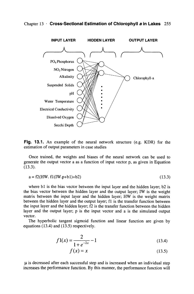
Fig. 13.1. An example of the neural network structure (e.g. KDR) for the
estimation of output parameters in case studies
Once trained, the weights and biases of the neural network can be used to
generate the output vector a as a function of input vector p, as given in Equation
(13.3).
a = f2(HW. fl(lW.p+bl)+b2)
(13.3)
where bl is the bias vector between the input layer and the hidden layer; b2 is
the bias vector between the hidden layer and the output layer; IW is the weight
matrix between the input layer and the hidden layer; HW is the weight matrix
between the hidden layer and the output layer; fl is the transfer function between
the input layer and the hidden layer; f2 is the transfer function between the hidden
layer and the output layer; p is the input vector and a is the simulated output
vector.
The hyperbolic tangent sigmoid function and linear function are given by
equations (13.4) and (13.5) respectively.
2
fl(x) =
2 - 1
1 + e- x
(13.4)
fex) = X
(13.5)
J.t is decreased after each successful step and is increased when an individual step
increases the performance function. By this manner, the performance function will
INPUTLAVER
P04 Phosphorus
N03 Nitrogen
Alkalinity
Suspended Solids
pR
Water Temperature
Electrical Conducti vity
Dissolved Oxygen
Secchi Depth
HIDDEN LAVER
OUTPUT LA VER
Chlorophyll-a
Fig. 13.1. An example of the neural network structure (e.g. KDR) for the
estimation of output parameters in case studies
Once trained, the weights and biases of the neural network can be used to
generate the output vector a as a function of input vector p, as given in Equation
(13.3).
a = f2(HW. fl(lW.p+bl)+b2)
(13.3)
where bl is the bias vector between the input layer and the hidden layer; b2 is
the bias vector between the hidden layer and the output layer; IW is the weight
matrix between the input layer and the hidden layer; HW is the weight matrix
between the hidden layer and the output layer; fl is the transfer function between
the input layer and the hidden layer; f2 is the transfer function between the hidden
layer and the output layer; p is the input vector and a is the simulated output
vector.
The hyperbolic tangent sigmoid function and linear function are given by
equations (13.4) and (13.5) respectively.
2
fl(x) =
2 - 1
1 + e- x
(13.4)
fex) = X
(13.5)
J.t is decreased after each successful step and is increased when an individual step
increases the performance function. By this manner, the performance function will