

Chapter 12 . Pattern Analysis 01 Endemie Fish Speeies in Rivers
237
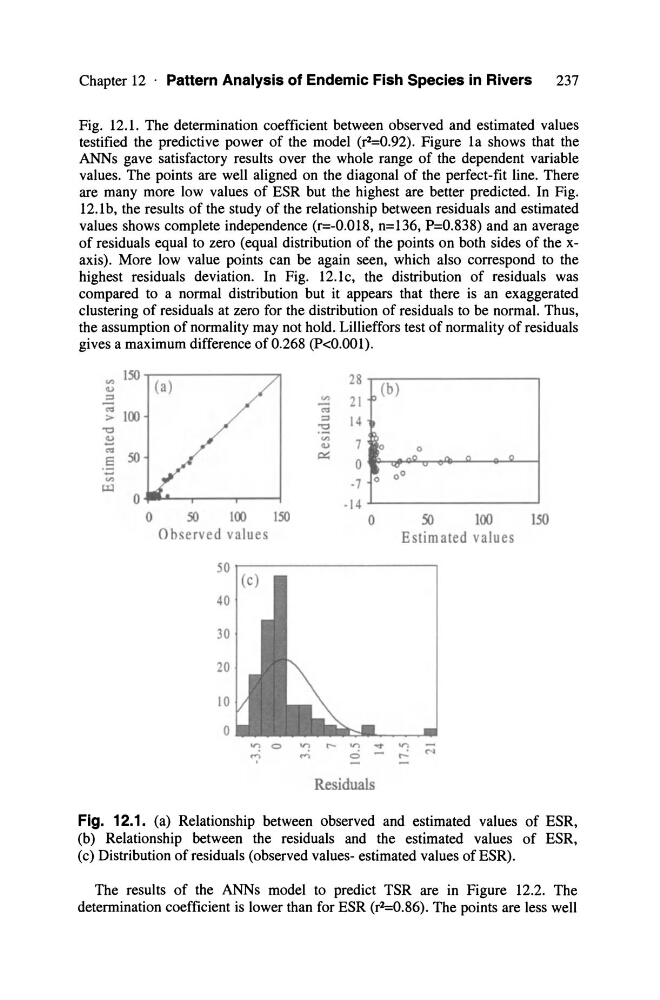
Fig. 12.1. The determination coefficient between observed and estimated values
testified the predictive power of the model (r2:0.92). Figure la shows that the
ANNs gave satisfactory results over the whole range of the dependent variable
values. The points are weIl aligned on the diagonal of the perfect-fit line. There
are many more low values of ESR but the highest are better predicted. In Fig.
12.1b, the results of the study of the relationship between residuals and estimated
values shows complete independence (r=-0.018, n=136, P=O.838) and an average
of residuals equal to zero (equal distribution of the points on both sides of the xaxis). More low value points can be again seen, wh ich also correspond to the
highest residuals deviation. In Fig. 12.1c, the distribution of residuals was
compared to a normal distribution but it appears that there is an exaggerated
clustering of residuals at zero for the distribution of residuals to be normal. Thus,
the assumption of normality may not hold. Lillieffors test of normality of residuals
gives a maximum difference of 0.268 (P
ISO
0
:::I
c;
100
>
"0
~
C':S
SO
.§
V>
UJ
0
0
(a)
28 p (b)
21
C':S
:::I
14
"0
'" 7
~
0
,0 0
p::;
0
n
0
~ ""0
v
-7
o 0
-14
SO
\00
\SO
0
50
100
Observed values
Estimated values
50,--------------------,
40
30
20
10
o
Residuals
150
Fig. 12.1. (a) Relationship between observed and estimated values of ESR,
(b) Relationship between the residuals and the estimated values of ESR,
(c) Distribution of residuals (observed values- estimated values of ESR).
The results of the ANNs model to predict TSR are in Figure 12.2. The
determination coefficient is lower than for ESR (r 2 =0.86). The points are less weIl
237
Fig. 12.1. The determination coefficient between observed and estimated values
testified the predictive power of the model (r2:0.92). Figure la shows that the
ANNs gave satisfactory results over the whole range of the dependent variable
values. The points are weIl aligned on the diagonal of the perfect-fit line. There
are many more low values of ESR but the highest are better predicted. In Fig.
12.1b, the results of the study of the relationship between residuals and estimated
values shows complete independence (r=-0.018, n=136, P=O.838) and an average
of residuals equal to zero (equal distribution of the points on both sides of the xaxis). More low value points can be again seen, wh ich also correspond to the
highest residuals deviation. In Fig. 12.1c, the distribution of residuals was
compared to a normal distribution but it appears that there is an exaggerated
clustering of residuals at zero for the distribution of residuals to be normal. Thus,
the assumption of normality may not hold. Lillieffors test of normality of residuals
gives a maximum difference of 0.268 (P
ISO
0
:::I
c;
100
>
"0
~
C':S
SO
.§
V>
UJ
0
0
(a)
28 p (b)
21
C':S
:::I
14
"0
'" 7
~
0
,0 0
p::;
0
n
0
~ ""0
v
-7
o 0
-14
SO
\00
\SO
0
50
100
Observed values
Estimated values
50,--------------------,
40
30
20
10
o
Residuals
150
Fig. 12.1. (a) Relationship between observed and estimated values of ESR,
(b) Relationship between the residuals and the estimated values of ESR,
(c) Distribution of residuals (observed values- estimated values of ESR).
The results of the ANNs model to predict TSR are in Figure 12.2. The
determination coefficient is lower than for ESR (r 2 =0.86). The points are less weIl