

Chapter 8· Analysis of Stream Macroinvertebrate Communities
149
were not included for training. Chironomus sp., Orthocladius sp., Cricolopus sp.,
Limnodrilus sp. and Erpobdella sp. were chosen. The first three species are
Chironomidae, while the fourth and fifth species belong to Oligochaeta and
Hirudinea, respectively. These selected Genera occurred consistently at the study
sites during the survey period. Data collected from March 1996 to March 1998
were used for the learning process, and a portion of sampies were set aside for
recognition (Chon et al. 2000b).
Densities of the selected 5 Genera in sampled communities were provided as
data sets for inputs with 1 - 5 time the delays, i.e., q = 1, 2, ... , 5. With each
delay, input nodes were correspondingly added. For example, if 5 Genera were
introduced with 2 time delays, 5 x 2 = 10 nodes were assigned for each input. The
input layer was subsequently interconnected to the hidden layer. Eight to thirty
nodes were used in the hidden layer. The number of nodes in the hidden layer was
determined based on experiences on obtaining convergence in training. The
number of output nodes was 5, equal to the number of selected Genera. Similar to
the static implementation, the internal state of the network, NET pJ ' was obtained by
linear summation of products of weights and output values of nodes in the hidden
layer over time. Subsequently, these values were adjusted in a nonlinear fashion,
logistic function in this case, to produce outputs, Y(I)PJ' as follows (Wasserman
1989; Zurada 1992, Haykin 1994):
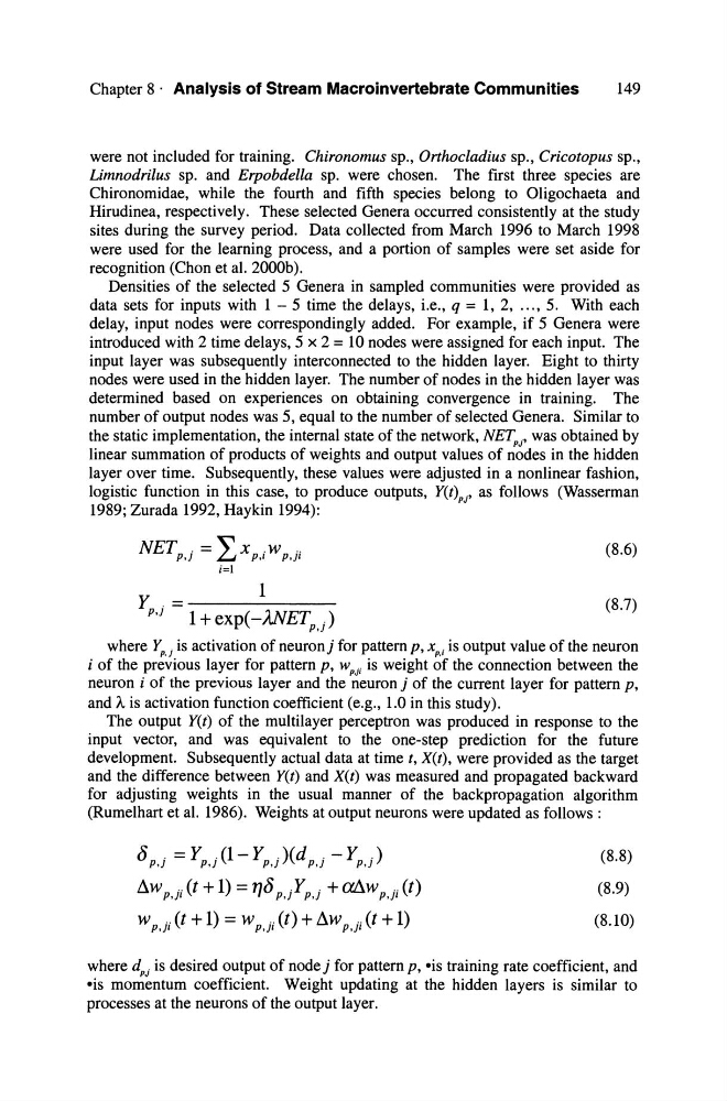
NETp,j = LX p,i W p,ji
(8.6)
i=1
1
Y . = - - - - - - -
P,}
1 + exp( -ANETp,j)
(8.7)
where Yp,J is activation of neuronj for patternp, Xp,i is output value of the neuron
i of the previous layer for pattern p, w pJi is weight of the connection between the
neuron i of the previous layer and the neuron j of the current layer for pattern p,
and A is activation function coefficient (e.g., 1.0 in this study).
The output Y(t) of the multilayer perceptron was produced in response to the
input vector, and was equivalent to the one-step prediction for the future
development. Subsequently actual data at time I, X(t), were provided as the target
and the difference between Y(I) and X(I) was measured and propagated backward
for adjusting weights in the usual manner of the backpropagation algorithm
(Rumelhart et al. 1986). Weights at output neurons were updated as folIows:
8 p,j = Yp,j (1- Yp,j )( d p,j - Yp,j )
ilw p,ji (t + 1) = 1]8 p,jYp,j + aL\w p,ji (t)
W p,ji (t + 1) = W p,ji (t) + ilw p,ji (t + 1)
(8.8)
(8.9)
(8.10)
where d pJ is desired output of node j for pattern p, eis training rate coefficient, and
eis momentum coefficient. Weight updating at the hidden layers is similar to
processes at the neurons of the output layer.
149
were not included for training. Chironomus sp., Orthocladius sp., Cricolopus sp.,
Limnodrilus sp. and Erpobdella sp. were chosen. The first three species are
Chironomidae, while the fourth and fifth species belong to Oligochaeta and
Hirudinea, respectively. These selected Genera occurred consistently at the study
sites during the survey period. Data collected from March 1996 to March 1998
were used for the learning process, and a portion of sampies were set aside for
recognition (Chon et al. 2000b).
Densities of the selected 5 Genera in sampled communities were provided as
data sets for inputs with 1 - 5 time the delays, i.e., q = 1, 2, ... , 5. With each
delay, input nodes were correspondingly added. For example, if 5 Genera were
introduced with 2 time delays, 5 x 2 = 10 nodes were assigned for each input. The
input layer was subsequently interconnected to the hidden layer. Eight to thirty
nodes were used in the hidden layer. The number of nodes in the hidden layer was
determined based on experiences on obtaining convergence in training. The
number of output nodes was 5, equal to the number of selected Genera. Similar to
the static implementation, the internal state of the network, NET pJ ' was obtained by
linear summation of products of weights and output values of nodes in the hidden
layer over time. Subsequently, these values were adjusted in a nonlinear fashion,
logistic function in this case, to produce outputs, Y(I)PJ' as follows (Wasserman
1989; Zurada 1992, Haykin 1994):
NETp,j = LX p,i W p,ji
(8.6)
i=1
1
Y . = - - - - - - -
P,}
1 + exp( -ANETp,j)
(8.7)
where Yp,J is activation of neuronj for patternp, Xp,i is output value of the neuron
i of the previous layer for pattern p, w pJi is weight of the connection between the
neuron i of the previous layer and the neuron j of the current layer for pattern p,
and A is activation function coefficient (e.g., 1.0 in this study).
The output Y(t) of the multilayer perceptron was produced in response to the
input vector, and was equivalent to the one-step prediction for the future
development. Subsequently actual data at time I, X(t), were provided as the target
and the difference between Y(I) and X(I) was measured and propagated backward
for adjusting weights in the usual manner of the backpropagation algorithm
(Rumelhart et al. 1986). Weights at output neurons were updated as folIows:
8 p,j = Yp,j (1- Yp,j )( d p,j - Yp,j )
ilw p,ji (t + 1) = 1]8 p,jYp,j + aL\w p,ji (t)
W p,ji (t + 1) = W p,ji (t) + ilw p,ji (t + 1)
(8.8)
(8.9)
(8.10)
where d pJ is desired output of node j for pattern p, eis training rate coefficient, and
eis momentum coefficient. Weight updating at the hidden layers is similar to
processes at the neurons of the output layer.