

296
scape analyses and the assessment of ecological
conditions (Hann et aI., 1997; Jensen et at, 1997).
For example, in the ICBEMP, the assessment area
was defined by an analysis of biophysical, ecological, and administrative maps in light of political
directives to develop an ecosystem management
strategy for forests east of the Cascade crest in the
U.S. Pacific Northwest (Figure 20.1) (Quigley and
Arbelbide, 1997). Provinces (sensu Bailey, 1995)
were used as the units for many biophysical and
vegetation analyses (Figure 20.1) (Jensen et aI.,
1997).
Delineation of assessment and analysis areas is
necessary because there is often a mismatch between traditional planning units and the boundaries
required by the objectives of an assessment (Knight
and Landres, 1998; Groom et aI., 1999). Traditional
planning units include such administrative boundaries as National Forests, National Parks, and counties, which historically were delineated without explicit consideration of ecosystem distribution,
functioning, and persistence.
20.3.2 Delineation of Land Units
Within assessment and analysis areas, a land unit
for RA is defined as the basic unit of selection for
inclusion in a network of conservation areas. Such
a land unit may contain more than one conservation target of interest (e.g., species, vegetation type,
ecosystem). Delineation of land units for RA follows the procedures of ecosystem characterization
(see Chapters 3, 22, and 23) and requires (l) characterization of biotic ecosystem components, (2)
characterization of environmental ecosystem components relevant to the biota, (3) characterization
of biotic-environmental interactions to define the
environmental space occupied by each biotic element, (4) characterization of ecosystems as a whole
and of ecosystem properties, and (5) a method of
mapping these components, interactions, and properties. Hierarchical databases (see Chapters 5 and
7) and classifications and maps of ecological and
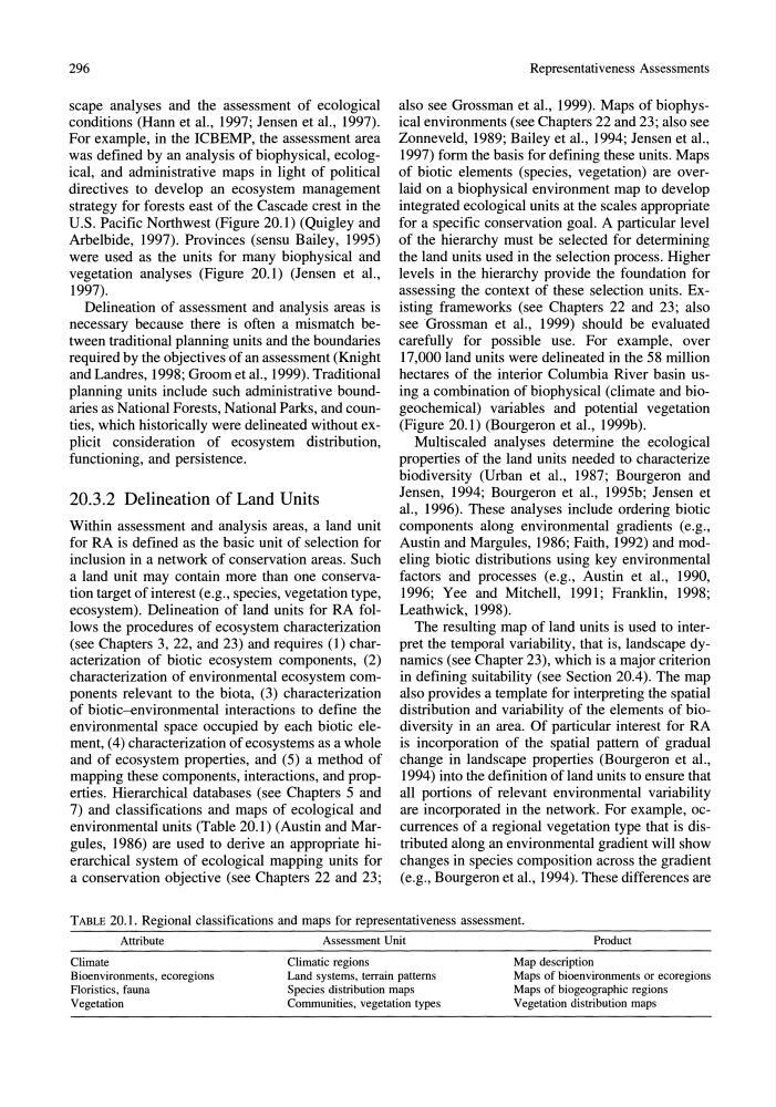
environmental units (Table 20.1) (Austin and Margules, 1986) are used to derive an appropriate hierarchical system of ecological mapping units for
a conservation objective (see Chapters 22 and 23;
Representativeness Assessments
also see Grossman et al., 1999). Maps of biophysical environments (see Chapters 22 and 23; also see
Zonneveld, 1989; Bailey et aI., 1994; Jensen et aI.,
1997) form the basis for defining these units. Maps
of biotic elements (species, vegetation) are overlaid on a biophysical environment map to develop
integrated ecological units at the scales appropriate
for a specific conservation goal. A particular level
of the hierarchy must be selected for determining
the land units used in the selection process. Higher
levels in the hierarchy provide the foundation for
assessing the context of these selection units. Existing frameworks (see Chapters 22 and 23; also
see Grossman et aI., 1999) should be evaluated
carefully for possible use. For example, over
17,000 land units were delineated in the 58 million
hectares of the interior Columbia River basin using a combination of biophysical (climate and biogeochemical) variables and potential vegetation
(Figure 20.1) (Bourgeron et aI., 1999b).
Multiscaled analyses determine the ecological
properties of the land units needed to characterize
biodiversity (Urban et aI., 1987; Bourgeron and
Jensen, 1994; Bourgeron et aI., 1995b; Jensen et
aI., 1996). These analyses include ordering biotic
components along environmental gradients (e.g.,
Austin and Margules, 1986; Faith, 1992) and modeling biotic distributions using key environmental
factors and processes (e.g., Austin et aI., 1990,
1996; Yee and Mitchell, 1991; Franklin, 1998;
Leathwick, 1998).
The resulting map of land units is used to interpret the temporal variability, that is, landscape dynamics (see Chapter 23), which is a major criterion
in defining suitability (see Section 20.4). The map
also provides a template for interpreting the spatial
distribution and variability of the elements of biodiversity in an area. Of particular interest for RA
is incorporation of the spatial pattern of gradual
change in landscape properties (Bourgeron et aI.,
1994) into the definition of land units to ensure that
all portions of relevant environmental variability
are incorporated in the network. For example, occurrences of a regional vegetation type that is distributed along an environmental gradient will show
changes in species composition across the gradient
(e.g., Bourgeron et aI., 1994). These differences are
TABLE 20.1. Regional classifications and maps for representativeness assessment.
Attribute
Assessment Unit
Product
Climate
Bioenvironments, ecoregions
Floristics, fauna
Vegetation
Climatic regions
Land systems, terrain patterns
Species distribution maps
Communities, vegetation types
Map description
Maps of bioenvironments or ecoregions
Maps of biogeographic regions
Vegetation distribution maps
scape analyses and the assessment of ecological
conditions (Hann et aI., 1997; Jensen et at, 1997).
For example, in the ICBEMP, the assessment area
was defined by an analysis of biophysical, ecological, and administrative maps in light of political
directives to develop an ecosystem management
strategy for forests east of the Cascade crest in the
U.S. Pacific Northwest (Figure 20.1) (Quigley and
Arbelbide, 1997). Provinces (sensu Bailey, 1995)
were used as the units for many biophysical and
vegetation analyses (Figure 20.1) (Jensen et aI.,
1997).
Delineation of assessment and analysis areas is
necessary because there is often a mismatch between traditional planning units and the boundaries
required by the objectives of an assessment (Knight
and Landres, 1998; Groom et aI., 1999). Traditional
planning units include such administrative boundaries as National Forests, National Parks, and counties, which historically were delineated without explicit consideration of ecosystem distribution,
functioning, and persistence.
20.3.2 Delineation of Land Units
Within assessment and analysis areas, a land unit
for RA is defined as the basic unit of selection for
inclusion in a network of conservation areas. Such
a land unit may contain more than one conservation target of interest (e.g., species, vegetation type,
ecosystem). Delineation of land units for RA follows the procedures of ecosystem characterization
(see Chapters 3, 22, and 23) and requires (l) characterization of biotic ecosystem components, (2)
characterization of environmental ecosystem components relevant to the biota, (3) characterization
of biotic-environmental interactions to define the
environmental space occupied by each biotic element, (4) characterization of ecosystems as a whole
and of ecosystem properties, and (5) a method of
mapping these components, interactions, and properties. Hierarchical databases (see Chapters 5 and
7) and classifications and maps of ecological and
environmental units (Table 20.1) (Austin and Margules, 1986) are used to derive an appropriate hierarchical system of ecological mapping units for
a conservation objective (see Chapters 22 and 23;
Representativeness Assessments
also see Grossman et al., 1999). Maps of biophysical environments (see Chapters 22 and 23; also see
Zonneveld, 1989; Bailey et aI., 1994; Jensen et aI.,
1997) form the basis for defining these units. Maps
of biotic elements (species, vegetation) are overlaid on a biophysical environment map to develop
integrated ecological units at the scales appropriate
for a specific conservation goal. A particular level
of the hierarchy must be selected for determining
the land units used in the selection process. Higher
levels in the hierarchy provide the foundation for
assessing the context of these selection units. Existing frameworks (see Chapters 22 and 23; also
see Grossman et aI., 1999) should be evaluated
carefully for possible use. For example, over
17,000 land units were delineated in the 58 million
hectares of the interior Columbia River basin using a combination of biophysical (climate and biogeochemical) variables and potential vegetation
(Figure 20.1) (Bourgeron et aI., 1999b).
Multiscaled analyses determine the ecological
properties of the land units needed to characterize
biodiversity (Urban et aI., 1987; Bourgeron and
Jensen, 1994; Bourgeron et aI., 1995b; Jensen et
aI., 1996). These analyses include ordering biotic
components along environmental gradients (e.g.,
Austin and Margules, 1986; Faith, 1992) and modeling biotic distributions using key environmental
factors and processes (e.g., Austin et aI., 1990,
1996; Yee and Mitchell, 1991; Franklin, 1998;
Leathwick, 1998).
The resulting map of land units is used to interpret the temporal variability, that is, landscape dynamics (see Chapter 23), which is a major criterion
in defining suitability (see Section 20.4). The map
also provides a template for interpreting the spatial
distribution and variability of the elements of biodiversity in an area. Of particular interest for RA
is incorporation of the spatial pattern of gradual
change in landscape properties (Bourgeron et aI.,
1994) into the definition of land units to ensure that
all portions of relevant environmental variability
are incorporated in the network. For example, occurrences of a regional vegetation type that is distributed along an environmental gradient will show
changes in species composition across the gradient
(e.g., Bourgeron et aI., 1994). These differences are
TABLE 20.1. Regional classifications and maps for representativeness assessment.
Attribute
Assessment Unit
Product
Climate
Bioenvironments, ecoregions
Floristics, fauna
Vegetation
Climatic regions
Land systems, terrain patterns
Species distribution maps
Communities, vegetation types
Map description
Maps of bioenvironments or ecoregions
Maps of biogeographic regions
Vegetation distribution maps