

information necessary to fully describe the clustering results and draw the
dendrogram. To display the list of items available in the output object, type
summary(object) where “object” is the clustering result.
This information can also be used to help interpret and compare clustering results.
We will now explore several possibilities offered by R for this purpose.
4.7.2 Cophenetic Correlation
The cophenetic distance between two objects in a dendrogram is the distance where
the two objects become members of the same group. Locate any two objects, start
from one, and “climb up the tree” to the first node leading down to the second object:
the level of that node along the distance scale is the cophenetic distance between the
two objects. A cophenetic matrix is a matrix representing the cophenetic distances
among all pairs of objects. A Pearson’s r correlation, called the cophenetic correlation in this context, can be computed between the original dissimilarity matrix and
the cophenetic matrix. The method with the highest cophenetic correlation may be
seen as the one that produces the clustering model that retains most of the information contained in the dissimilarity matrix. This does not necessarily mean, however,
that this clustering model is the most adequate for the researcher’s goal.
Of course, the cophenetic correlation cannot be tested for significance, since the
cophenetic matrix is derived from the original dissimilarity matrix. The two sets of
distances are not independent. Furthermore, the cophenetic correlation depends
strongly on the clustering method used, in addition to the data.
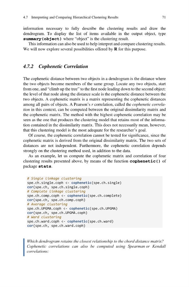
As an example, let us compute the cophenetic matrix and correlation of four
clustering results presented above, by means of the function cophenetic() of
package stats.
# Single linkage clustering
spe.ch.single.coph <- cophenetic(spe.ch.single)
cor(spe.ch, spe.ch.single.coph)
# Complete linkage clustering
spe.ch.comp.coph <- cophenetic(spe.ch.complete)
cor(spe.ch, spe.ch.comp.coph)
# Average clustering
spe.ch.UPGMA.coph <- cophenetic(spe.ch.UPGMA)
cor(spe.ch, spe.ch.UPGMA.coph)
# Ward clustering
spe.ch.ward.coph <- cophenetic(spe.ch.ward)
cor(spe.ch, spe.ch.ward.coph)
Which dendrogram retains the closest relationship to the chord distance matrix?
Cophenetic correlations can also be computed using Spearman or Kendall
correlations:
4.7 Interpreting and Comparing Hierarchical Clustering Results
71
dendrogram. To display the list of items available in the output object, type
summary(object) where “object” is the clustering result.
This information can also be used to help interpret and compare clustering results.
We will now explore several possibilities offered by R for this purpose.
4.7.2 Cophenetic Correlation
The cophenetic distance between two objects in a dendrogram is the distance where
the two objects become members of the same group. Locate any two objects, start
from one, and “climb up the tree” to the first node leading down to the second object:
the level of that node along the distance scale is the cophenetic distance between the
two objects. A cophenetic matrix is a matrix representing the cophenetic distances
among all pairs of objects. A Pearson’s r correlation, called the cophenetic correlation in this context, can be computed between the original dissimilarity matrix and
the cophenetic matrix. The method with the highest cophenetic correlation may be
seen as the one that produces the clustering model that retains most of the information contained in the dissimilarity matrix. This does not necessarily mean, however,
that this clustering model is the most adequate for the researcher’s goal.
Of course, the cophenetic correlation cannot be tested for significance, since the
cophenetic matrix is derived from the original dissimilarity matrix. The two sets of
distances are not independent. Furthermore, the cophenetic correlation depends
strongly on the clustering method used, in addition to the data.
As an example, let us compute the cophenetic matrix and correlation of four
clustering results presented above, by means of the function cophenetic() of
package stats.
# Single linkage clustering
spe.ch.single.coph <- cophenetic(spe.ch.single)
cor(spe.ch, spe.ch.single.coph)
# Complete linkage clustering
spe.ch.comp.coph <- cophenetic(spe.ch.complete)
cor(spe.ch, spe.ch.comp.coph)
# Average clustering
spe.ch.UPGMA.coph <- cophenetic(spe.ch.UPGMA)
cor(spe.ch, spe.ch.UPGMA.coph)
# Ward clustering
spe.ch.ward.coph <- cophenetic(spe.ch.ward)
cor(spe.ch, spe.ch.ward.coph)
Which dendrogram retains the closest relationship to the chord distance matrix?
Cophenetic correlations can also be computed using Spearman or Kendall
correlations:
4.7 Interpreting and Comparing Hierarchical Clustering Results
71