

The same variables are now compared using Kendall’s τ:
# Kendall tau rank correlation among environmental variables,
# no colours
env.ken <- cor(env, method = "kendall")
env.o <- order.single(env.ken)
pairs(env[ ,env.o], lower.panel = panel.smoothb,
upper.panel = panel.cor, no.col = TRUE,
method = "kendall", diag.panel = panel.hist,
main = "Kendall Correlation Matrix")
bod
0 2 4
0.909
***
0.903
***
0 2 4 6
0.683
***
0.435
*
0 30 70
0.295
0.337
.
7.8 8.4
-0.162
-0.84
***
200 800
-0.383
*
5
15
-0.174
0 2 4
pho
0.97
***
0.801
***
0.473
**
0.379
*
0.373
*
-0.079
-0.758
***
-0.437
*
-0.195
amm 0.802
***
0.408
*
0.293
0.296
-0.122
-0.746
***
-0.381
*
0.0 1.5
-0.175
0 3 6
nit
0.738
***
0.593
***
0.535
**
-0.04
-0.687
***
-0.753
***
-0.314
.
dfs
0.947
***
0.733
***
0.016
-0.57
**
-0.938
***
0 300
-0.395
*
0 30 70
dis
0.737
***
0.033
-0.421
*
-0.863
***
-0.358
.
har
0.085
-0.374
*
-0.786
***
40 80
-0.527
**
7.8 8.4
pH
0.192
-0.05
-0.222
oxy
0.425
*
4
8 12
0.308
200 800
ele
0.457
*
0 20
slo
Pearson Correlation Matrix
5 15
0.0 1.0
0 300
40 80
4 8 12
0 20
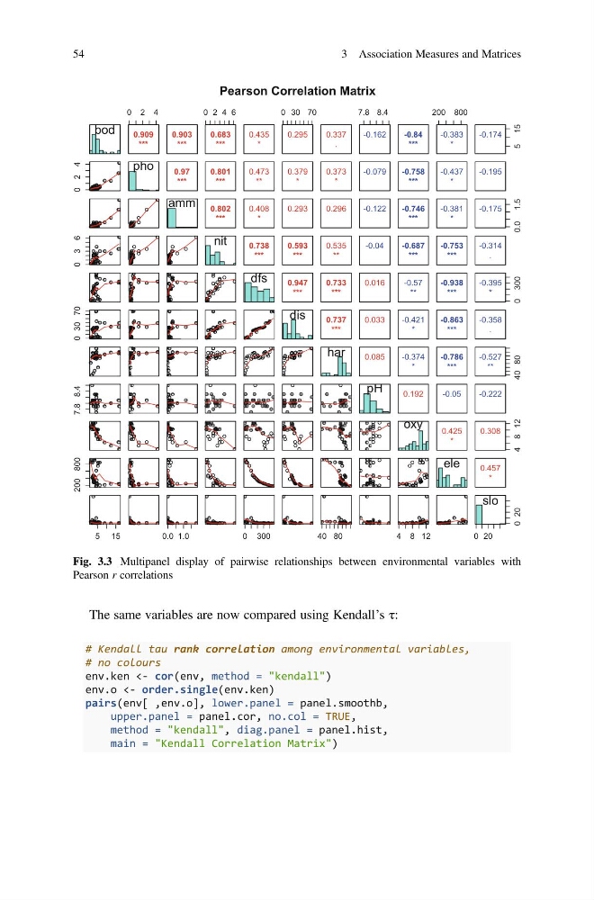
Fig. 3.3 Multipanel display of pairwise relationships between environmental variables with
Pearson r correlations
54
3 Association Measures and Matrices
# Kendall tau rank correlation among environmental variables,
# no colours
env.ken <- cor(env, method = "kendall")
env.o <- order.single(env.ken)
pairs(env[ ,env.o], lower.panel = panel.smoothb,
upper.panel = panel.cor, no.col = TRUE,
method = "kendall", diag.panel = panel.hist,
main = "Kendall Correlation Matrix")
bod
0 2 4
0.909
***
0.903
***
0 2 4 6
0.683
***
0.435
*
0 30 70
0.295
0.337
.
7.8 8.4
-0.162
-0.84
***
200 800
-0.383
*
5
15
-0.174
0 2 4
pho
0.97
***
0.801
***
0.473
**
0.379
*
0.373
*
-0.079
-0.758
***
-0.437
*
-0.195
amm 0.802
***
0.408
*
0.293
0.296
-0.122
-0.746
***
-0.381
*
0.0 1.5
-0.175
0 3 6
nit
0.738
***
0.593
***
0.535
**
-0.04
-0.687
***
-0.753
***
-0.314
.
dfs
0.947
***
0.733
***
0.016
-0.57
**
-0.938
***
0 300
-0.395
*
0 30 70
dis
0.737
***
0.033
-0.421
*
-0.863
***
-0.358
.
har
0.085
-0.374
*
-0.786
***
40 80
-0.527
**
7.8 8.4
pH
0.192
-0.05
-0.222
oxy
0.425
*
4
8 12
0.308
200 800
ele
0.457
*
0 20
slo
Pearson Correlation Matrix
5 15
0.0 1.0
0 300
40 80
4 8 12
0 20
Fig. 3.3 Multipanel display of pairwise relationships between environmental variables with
Pearson r correlations
54
3 Association Measures and Matrices