

# Remove the 'dfs' variable from the env dataset
env2 <- env[,-1]
# Euclidean distance matrix of the standardized env2 data frame
env.de <- dist(scale(env2))
coldiss(env.de, nc = 16, diag = TRUE)
Hint See how the environmental variables have been standardized “on the fly” using
the function scale().
Such plots of dissimilarity matrices can be used for a quick comparison. For
instance, you could plot the Hellinger species-based distance matrix and the environmental distance matrix, both using equal-sized categories (byrank ¼ TRUE, the
default), in order to compare them visually:
# Hellinger distance matrix of the species data
# Use nc = 16 equal-sized classes
coldiss(spe.dh, nc = 16, diag = TRUE)
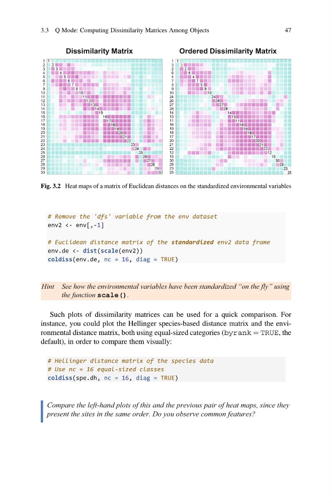
Compare the left-hand plots of this and the previous pair of heat maps, since they
present the sites in the same order. Do you observe common features?
Dissimilarity Matrix
30
29
28
27
26
25
24
23
22
21
20
19
18
17
16
15
14
13
12
11
10
9
7
6
5
4
3
2
1 1
2
3
4
5
6
7
9
10
11
12
13
14
15
16
17
18
19
20
21
22
23
24
25
26
27
28
29
30
Ordered Dissimilarity Matrix
25
23
29
30
15
12
22
21
20
17
18
19
16
11
13
14
28
27
26
24
10
9
5
7
4
6
2
3
1 1
3
2
6
4
7
5
9
10
24
26
27
28
14
13
11
16
19
18
17
20
21
22
12
15
30
29
23
25
Fig. 3.2 Heat maps of a matrix of Euclidean distances on the standardized environmental variables
3.3 Q Mode: Computing Dissimilarity Matrices Among Objects
47
env2 <- env[,-1]
# Euclidean distance matrix of the standardized env2 data frame
env.de <- dist(scale(env2))
coldiss(env.de, nc = 16, diag = TRUE)
Hint See how the environmental variables have been standardized “on the fly” using
the function scale().
Such plots of dissimilarity matrices can be used for a quick comparison. For
instance, you could plot the Hellinger species-based distance matrix and the environmental distance matrix, both using equal-sized categories (byrank ¼ TRUE, the
default), in order to compare them visually:
# Hellinger distance matrix of the species data
# Use nc = 16 equal-sized classes
coldiss(spe.dh, nc = 16, diag = TRUE)
Compare the left-hand plots of this and the previous pair of heat maps, since they
present the sites in the same order. Do you observe common features?
Dissimilarity Matrix
30
29
28
27
26
25
24
23
22
21
20
19
18
17
16
15
14
13
12
11
10
9
7
6
5
4
3
2
1 1
2
3
4
5
6
7
9
10
11
12
13
14
15
16
17
18
19
20
21
22
23
24
25
26
27
28
29
30
Ordered Dissimilarity Matrix
25
23
29
30
15
12
22
21
20
17
18
19
16
11
13
14
28
27
26
24
10
9
5
7
4
6
2
3
1 1
3
2
6
4
7
5
9
10
24
26
27
28
14
13
11
16
19
18
17
20
21
22
12
15
30
29
23
25
Fig. 3.2 Heat maps of a matrix of Euclidean distances on the standardized environmental variables
3.3 Q Mode: Computing Dissimilarity Matrices Among Objects
47