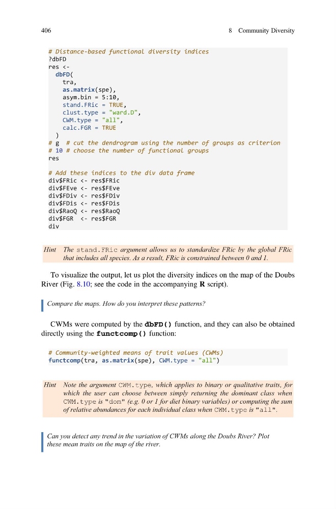
# Distance-based functional diversity indices
?dbFD
res tra,
as.matrix(spe),
asym.bin = 5:10,
stand.FRic = TRUE,
clust.type = "ward.D",
CWM.type = "all",
calc.FGR = TRUE
)
# g # cut the dendrogram using the number of groups as criterion
# 10 # choose the number of functional groups
res
# Add these indices to the div data frame
div$FRic <- res$FRic
div$FEve <- res$FEve
div$FDiv <- res$FDiv
div$FDis <- res$FDis
div$RaoQ <- res$RaoQ
div$FGR <- res$FGR
div
Hint The stand.FRic argument allows us to standardize FRic by the global FRic
that includes all species. As a result, FRic is constrained between 0 and 1.
To visualize the output, let us plot the diversity indices on the map of the Doubs
River (Fig. 8.10; see the code in the accompanying R script).
Compare the maps. How do you interpret these patterns?
CWMs were computed by the dbFD() function, and they can also be obtained
directly using the functcomp() function:
# Community-weighted means of trait values (CWMs)
functcomp(tra, as.matrix(spe), CWM.type = "all")
Hint Note the argument CWM.type, which applies to binary or qualitative traits, for
which the user can choose between simply returning the dominant class when
CWM.type is "dom" (e.g. 0 or 1 for diet binary variables) or computing the sum
of relative abundances for each individual class when CWM.type is "all".
Can you detect any trend in the variation of CWMs along the Doubs River? Plot
these mean traits on the map of the river.
406
8 Community Diversity