

The first db-RDA result (replacement) shows a very weak relationship of the
replacement matrix with the environmental variables (R
2
adj ¼ 0.038, p ¼ 0.007). It is
not advisable to apply this analysis to strongly non-Euclidean matrices, as it is the
case for most Repl matrices. We will refrain from drawing a biplot, which might give
a false impression of containing useful information. On the other hand, richness
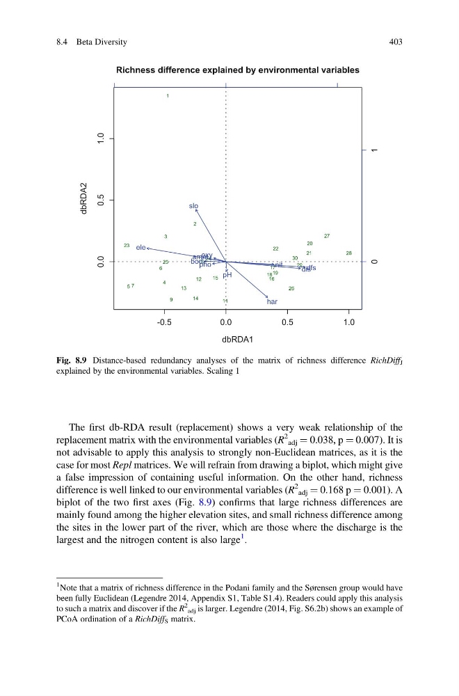
difference is well linked to our environmental variables (R
2
adj ¼ 0.168 p ¼ 0.001). A
biplot of the two first axes (Fig. 8.9) confirms that large richness differences are
mainly found among the higher elevation sites, and small richness difference among
the sites in the lower part of the river, which are those where the discharge is the
largest and the nitrogen content is also large
1 .
-0.5
0.0
0.5
1.0
0.0
0.5
1.0
Richness difference explained by environmental variables
dbRDA1
dbRDA2
1
2
3
4
5
6
7
9
10
11
12
13
14
15
16
17
18 19
20
21
22
23
24
25
26
27
28
29
30
dfs
ele
slo
dis
pH
har
pho
nit
amm oxy
bod
0
1
Fig. 8.9 Distance-based redundancy analyses of the matrix of richness difference RichDiff J
explained by the environmental variables. Scaling 1
1 Note that a matrix of richness difference in the Podani family and the Sørensen group would have
been fully Euclidean (Legendre 2014, Appendix S1, Table S1.4). Readers could apply this analysis
to such a matrix and discover if the R
2
adj is larger. Legendre (2014, Fig. S6.2b) shows an example of
PCoA ordination of a RichDiff S matrix.
8.4 Beta Diversity
403
replacement matrix with the environmental variables (R
2
adj ¼ 0.038, p ¼ 0.007). It is
not advisable to apply this analysis to strongly non-Euclidean matrices, as it is the
case for most Repl matrices. We will refrain from drawing a biplot, which might give
a false impression of containing useful information. On the other hand, richness
difference is well linked to our environmental variables (R
2
adj ¼ 0.168 p ¼ 0.001). A
biplot of the two first axes (Fig. 8.9) confirms that large richness differences are
mainly found among the higher elevation sites, and small richness difference among
the sites in the lower part of the river, which are those where the discharge is the
largest and the nitrogen content is also large
1 .
-0.5
0.0
0.5
1.0
0.0
0.5
1.0
Richness difference explained by environmental variables
dbRDA1
dbRDA2
1
2
3
4
5
6
7
9
10
11
12
13
14
15
16
17
18 19
20
21
22
23
24
25
26
27
28
29
30
dfs
ele
slo
dis
pH
har
pho
nit
amm oxy
bod
0
1
Fig. 8.9 Distance-based redundancy analyses of the matrix of richness difference RichDiff J
explained by the environmental variables. Scaling 1
1 Note that a matrix of richness difference in the Podani family and the Sørensen group would have
been fully Euclidean (Legendre 2014, Appendix S1, Table S1.4). Readers could apply this analysis
to such a matrix and discover if the R
2
adj is larger. Legendre (2014, Fig. S6.2b) shows an example of
PCoA ordination of a RichDiff S matrix.
8.4 Beta Diversity
403