

(2) total replacement diversity, (3) total richness diversity (or nestedness), (4) total
replacement diversity/ BD Total , (5) total richness diversity (or nestedness)/ BD Total .
A final item ($note) gives the name of the dissimilarity coefficient.
In addition to beta.div.comp(), function LCBD.comp() found in
adespatial allows users to compute the total variance (BDtotal) associated
with any dissimilarity matrix with class “dist”, or any similar matrix representing
an additive decomposition of BDtotal into Repl, RichDiff, Nes or other components,
computed by other R functions. The function also computes the LCBD indices
derived from that matrix.
The diversities associated to the Jaccard D matrix and its Repl J and RichDiff J
components are computed on square-rooted values because the Jaccard dissimilarity
is not Euclidean but its square-root is. Calculation of total diversities is done by
computing SS Total and BD Total from a D matrix, as in Eqs. 8.13 and 8.11.
In our example, the vector of global results gives the following numbers:
[1] 0.3258676 0.0925460 0.2333216 0.2839988 0.7160012
It is easy to verify that the sum of the second and third values ¼ (rounded)
0.09 + 0.23 ¼ 0.32, i.e., that total replacement diversity and total richness diversity
sum to BD Total . In this example, the total richness diversity accounts for the larger
proportion (71.6%) of BD Total .
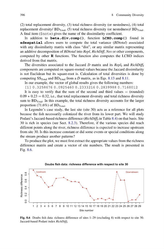
In Legendre’s case study, the last site (site 30) acts as a reference for all plots
because the fish necessarily colonized the river from its lower part. We will study
Podani’s Jaccard-based richness difference (RichDiff J in Table 8.4) on that basis. Site
30 is rich in species (see Sect. 8.2.3). Therefore, if the various species did reach
different points along the river, richness difference is expected to increase upstream
from site 30. Is this increase constant or did some events or special conditions along
the stream produce another patterns?
To produce the plot, we must first extract the appropriate values from the richness
difference matrix and create a vector of site numbers. The result is presented in
Fig. 8.6.
1 2 3 4 5 6 7 8 9 10 11 12 13 14 15 16 17 18 19 20 21 22 23 24 25 26 27 28 29
0.0 0.2 0.4 0.6 0.8
Doubs fish data: richness difference with respect to site 30
Site number
Richness difference
Upstream
Downstream
Fig. 8.6 Doubs fish data: richness difference of sites 1–29 (excluding 8) with respect to site 30.
Jaccard-based Podani index RichDiff J
396
8 Community Diversity
replacement diversity/ BD Total , (5) total richness diversity (or nestedness)/ BD Total .
A final item ($note) gives the name of the dissimilarity coefficient.
In addition to beta.div.comp(), function LCBD.comp() found in
adespatial allows users to compute the total variance (BDtotal) associated
with any dissimilarity matrix with class “dist”, or any similar matrix representing
an additive decomposition of BDtotal into Repl, RichDiff, Nes or other components,
computed by other R functions. The function also computes the LCBD indices
derived from that matrix.
The diversities associated to the Jaccard D matrix and its Repl J and RichDiff J
components are computed on square-rooted values because the Jaccard dissimilarity
is not Euclidean but its square-root is. Calculation of total diversities is done by
computing SS Total and BD Total from a D matrix, as in Eqs. 8.13 and 8.11.
In our example, the vector of global results gives the following numbers:
[1] 0.3258676 0.0925460 0.2333216 0.2839988 0.7160012
It is easy to verify that the sum of the second and third values ¼ (rounded)
0.09 + 0.23 ¼ 0.32, i.e., that total replacement diversity and total richness diversity
sum to BD Total . In this example, the total richness diversity accounts for the larger
proportion (71.6%) of BD Total .
In Legendre’s case study, the last site (site 30) acts as a reference for all plots
because the fish necessarily colonized the river from its lower part. We will study
Podani’s Jaccard-based richness difference (RichDiff J in Table 8.4) on that basis. Site
30 is rich in species (see Sect. 8.2.3). Therefore, if the various species did reach
different points along the river, richness difference is expected to increase upstream
from site 30. Is this increase constant or did some events or special conditions along
the stream produce another patterns?
To produce the plot, we must first extract the appropriate values from the richness
difference matrix and create a vector of site numbers. The result is presented in
Fig. 8.6.
1 2 3 4 5 6 7 8 9 10 11 12 13 14 15 16 17 18 19 20 21 22 23 24 25 26 27 28 29
0.0 0.2 0.4 0.6 0.8
Doubs fish data: richness difference with respect to site 30
Site number
Richness difference
Upstream
Downstream
Fig. 8.6 Doubs fish data: richness difference of sites 1–29 (excluding 8) with respect to site 30.
Jaccard-based Podani index RichDiff J
396
8 Community Diversity