# Construction of 5 fictitious species
# Two randomly distributed species
sp12 <- matrix(trunc(rnorm(80,5,2),0),40)
# One species restricted to the upper half of the stream
sp3 <- c(trunc(rnorm(20,8,2.5),0), rep(0,20))
# One species restricted to the left-hand half of the transect
sp4 <- t(matrix(c(trunc(rnorm(20,8,3),0), rep(0,20)),10))
sp4 <- as.vector(sp4)
# One species restricted to the 4 upper left-hand sites
sp5 <- c(4,7,0,0,3,8, rep(0,34))
# Build the species matrix
sp <- cbind(sp12, sp3, sp4, sp5)
colnames(sp) <- c("sp1", "sp2", "sp3", "sp4", "sp5")
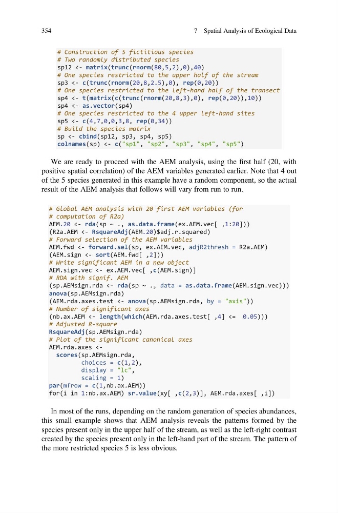
We are ready to proceed with the AEM analysis, using the first half (20, with
positive spatial correlation) of the AEM variables generated earlier. Note that 4 out
of the 5 species generated in this example have a random component, so the actual
result of the AEM analysis that follows will vary from run to run.
# Global AEM analysis with 20 first AEM variables (for
# computation of R2a)
AEM.20 <- rda(sp ~ ., as.data.frame(ex.AEM.vec[ ,1:20]))
(R2a.AEM <- RsquareAdj(AEM.20)$adj.r.squared)
# Forward selection of the AEM variables
AEM.fwd <- forward.sel(sp, ex.AEM.vec, adjR2thresh = R2a.AEM)
(AEM.sign <- sort(AEM.fwd[ ,2]))
# Write significant AEM in a new object
AEM.sign.vec <- ex.AEM.vec[ ,c(AEM.sign)]
# RDA with signif. AEM
(sp.AEMsign.rda <- rda(sp ~ ., data = as.data.frame(AEM.sign.vec)))
anova(sp.AEMsign.rda)
(AEM.rda.axes.test <- anova(sp.AEMsign.rda, by = "axis"))
# Number of significant axes
(nb.ax.AEM <- length(which(AEM.rda.axes.test[ ,4] <= 0.05)))
# Adjusted R-square
RsquareAdj(sp.AEMsign.rda)
# Plot of the significant canonical axes
AEM.rda.axes choices = c(1,2),
display = "lc",
scaling = 1)
par(mfrow = c(1,nb.ax.AEM))
for(i in 1:nb.ax.AEM) sr.value(xy[ ,c(2,3)], AEM.rda.axes[ ,i])
In most of the runs, depending on the random generation of species abundances,
this small example shows that AEM analysis reveals the patterns formed by the
species present only in the upper half of the stream, as well as the left-right contrast
created by the species present only in the left-hand part of the stream. The pattern of
the more restricted species 5 is less obvious.
354
7 Spatial Analysis of Ecological Data